This is an introduction into the complex number arithmetic of Euler. Most numerical functions are defined for complex numbers too.
>z=1+1i; exp(z^2)
-0.416147+0.909297i
The log function needs some care, since it is defined only for the plane without the negative axis. It is not continuous across the negative axis.
>log(-1+0.1i), log(-1-0.1i)
0.00497517+3.04192i
0.00497517-3.04192i
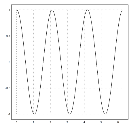
We can plot the real part of a complex curve as usual.
>plot2d("re(exp(3*I*x))",a=0,b=2*pi):
The arg function computes the argument of a complex number. It is, of course, discontinuous.
>plot2d("arg(exp(3*1i*x))",a=0,b=2*pi):
Numerical integration in Euler will work just as in the real case. However, complex integration along a path is defined differently.
![]()
>function gam(t) &= cos(t)+I*sin(t)
I sin(t) + cos(t)
>function dgam(t) &= -sin(t)+I*cos(t)
I cos(t) - sin(t)
>function f(z) &= 1/z
                                  1
                                  -
                                  z
Now we can integrate f around the unit circle. The exact result is 1.
>romberg("f(gam(x))*dgam(x)",0,2*pi)/(2*pi*I)
1+0i
If the function is analytic, the exact result should be 0.
>function f(z) &= 1/(z+2)^2
                                  1
                               --------
                                      2
                               (z + 2)
>romberg("f(gam(x))*dgam(x)",0,2*pi)/(2*pi*I)
0+0i
With these symbolic expressions, the result can be computed by Maxima.
>&integrate(f(gam(t))*dgam(t),t,0,2*pi)
0
For an example, let us compute the anti-derivative of a complex function in the complex plane by integration along the straight path from (0,0) to (a,b).
![]()
>function gam(t,a,b) &= t*a+I*t*b
I b t + a t
>function dgam(t,a,b) &= a+I*b
I b + a
>function f(z) &= exp(-z^2)
                                    2
                                 - z
                                E
E.g. in 1+2i
>romberg("f(gam(x,1,2))*dgam(x,1,2)",0,1)
-0.475588-4.47469i
The symbolic result is expressed in terms of the Gauß error function. This function is not implemented numerically in Euler or Maxima for complex values.
>&integrate(f(gam(t,1,2))*dgam(t,1,2),t)
               sqrt(pi) (2 I + 1) erf(sqrt(4 I - 3) t)
               ---------------------------------------
                           2 sqrt(4 I - 3)
We can also create function tables of complex functions along a curve.
In this example, let us generate 500 points distributed around the unit circle.
>z=exp(1i*linspace(0,2*pi,100));
Now we can plot the imge of the circle under the exp function easily.
>plot2d(exp(z),a=0,b=4,c=-2,d=2):
We can also plot the complete image of the unit circle under this mapping.
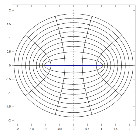
First we need to define a row vector of radii from 0 to 1 and a column vector of angles from 0 to 2pi.
>r=linspace(0,1,190); phi=linspace(0,2*pi,800)';
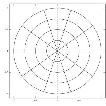
We can now generate a grid covering the unit circle, and we can plot it easily.
The plot2d function plots the grid. By default all grid points are plotted. But we can also specify any number of grid points with cgrid=... For a smooth look this number should divide the number of points evenly.
grid=1 simply turns off the coordinate grid.
>z=r*exp(phi*I); plot2d(z,a=-1,b=1,c=-1,d=1,grid=6,cgrid=[10,4]):
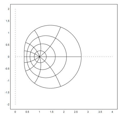
Now we plot the image of this grid under the exp function.
>plot2d(exp(z),a=0,b=4,c=-2,d=2,grid=1,cgrid=[10,4]):
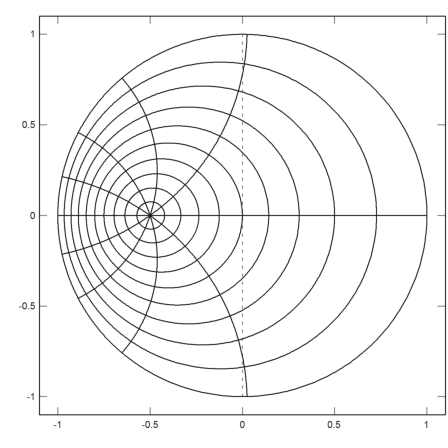
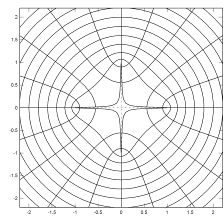
The following plot shows a conformal mapping from the unit circle to itself.
![]()
>plot2d((z-0.5)/(1-0.5*z),a=-1,b=1,c=-1,d=1,grid=6,cgrid=10):
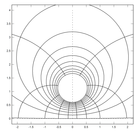
The following is the Joukowski mapping, which maps the outside of the unit circle onto the outside of the unit interval [-1,1] one-to-one.
>function J(z) := (z+1/z)/2
We wish to show the mapping outside of the unit circle. So we need to generate a grid there.
>z=linspace(1.01,4,100)*exp(1i*linspace(0,2*pi,400)');
First we look at the grid.
>plot2d(z,a=-2,b=2,c=-2,d=2,grid=2,cgrid=[20,10]):
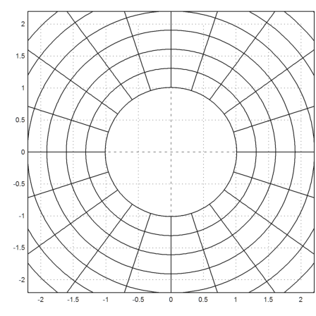
We map the grid and plot the result, adding the interval [-1,1] in thick blue.
>plot2d(J(z),a=-2,b=2,c=-2,d=2,grid=6,cgrid=10);  ...
   plot2d([-1,1],0,color=blue,thickness=3,add=true):
Let us define the inverse of the Joukowski mapping. We have to use cases here.
>function map invJ(z) ...
 w=sqrt(z^2-1);
 return z+(re(z)>=0)*w-(re(z)<0)*w;
 endfunction
You can compute the two branches symbolically.
>&solve((z+1/z)/2=w,z)
                            2                 2
             [z = w - sqrt(w  - 1), z = sqrt(w  - 1) + w]
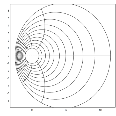
Using these functions, we can map the outside of the unit circle to the outside of a cross.
![]()
>plot2d(J(I*invJ(J(z)*sqrt(2))),a=-2,b=2,c=-2,d=2,grid=6,cgrid=[20,10]):
The following function maps the outside of the unit circle to the upper half plane.
![]()
>function H(z) &= (I*z+1)/(I+z)
                               I z + 1
                               -------
                                z + I
We can view the image of our grid. Note that infinity is mapped to i.
>plot2d(H(z),a=-2,b=2,c=0,d=4,grid=6,cgrid=10):
This is the inverse function, mapping the upper half plane to the outside of the unit circle.
>function invH(z) &= (I*z-1)/(I-z)
                               I z - 1
                               -------
                                I - z
Indeed.
>&solve(w=H(z),z)
                                 1 - I w
                            [z = -------]
                                  w - I
>invH(H(2)), invH(H(1i))
2+0i
0+1i
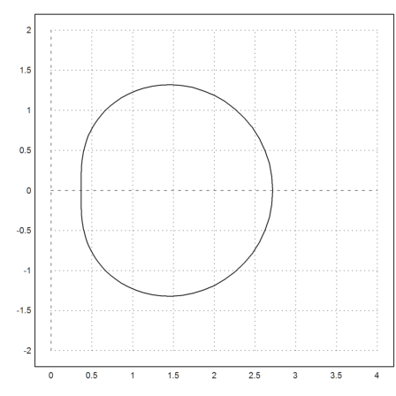
The next function maps the outside of the unit circle onto itself, and takes a to infinity.
![]()
>function L(z,a) := (a/conj(a))*(conj(a)*z-1)/(a-z)
In the following picture, 6 goes to infinity.
>plot2d(L(z,6),grid=1,cgrid=10):
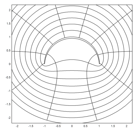
Now we map the outside of the unit circle to the outside of the arc with angle Pi.
![]()
>plot2d(invH(J(L(z,-invJ(1i)))),a=-2,b=2,c=-2,d=2,grid=4,cgrid=10):
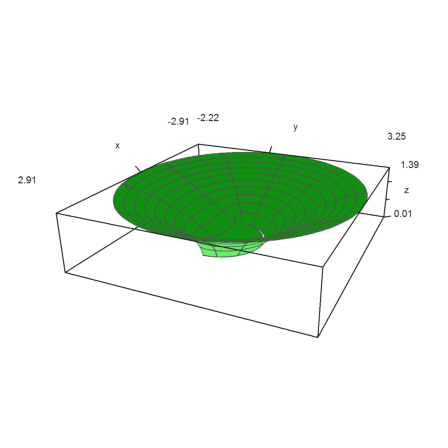
Let us plot the Green function of this arc in 3d.
>w=invH(J(L(z,-invJ(1i))));
>plot3d(re(w),im(w),log(abs(z)),scale=1.2,grid=10):
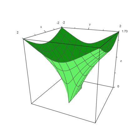
We take a grid around the interval [-1,1] and compute the Green function of each element of the Grid. Then we plot it in 3D.
>plot3d("log(abs(invJ(x+1i*y)))",xmin=-2,xmax=2,ymin=-2,ymax=2):
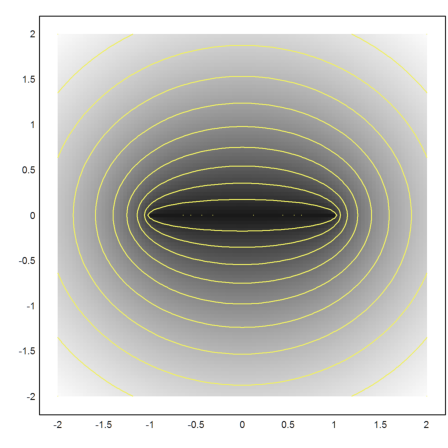
We can also get the level lines of this function.
>plot2d("log(abs(invJ(x+1i*y)))",r=2,n=100,>levels,hue=1, ...
   contourcolor=yellow,grid=4):
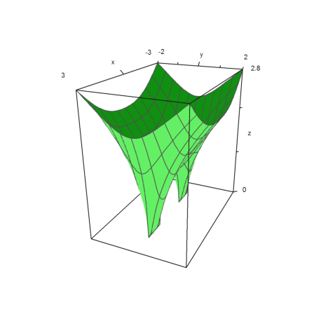
Here is the Green function of two intervals.
![]()
>plot3d("log(abs(invJ(((x+1i*y)^2-2.5)/1.5)))", ...
   xmin=-3,xmax=3,ymin=-2,ymax=2):
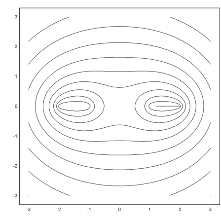
And its contour.
>plot2d("log(abs(invJ(((x+1i*y)^2-2.5)/1.5)))", ...
   n=100,r=3,>levels,grid=4,cgrid=10):
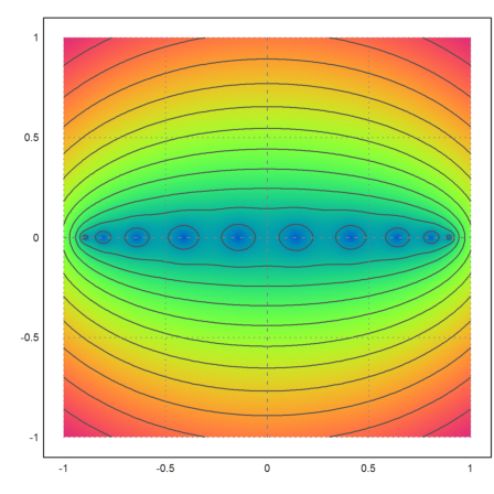
The following computes the Chebyshev polynomial in the complex plane, and draws a colorful image of the zeros.
>x=-1.1:0.01:1.1; y=x'; z=x+I*y; ...
 p=chebpoly(10); w=abs(evalpoly(z,p)); ...
 plot2d(log(w+0.2),level=0:10,>hue,>spectral):
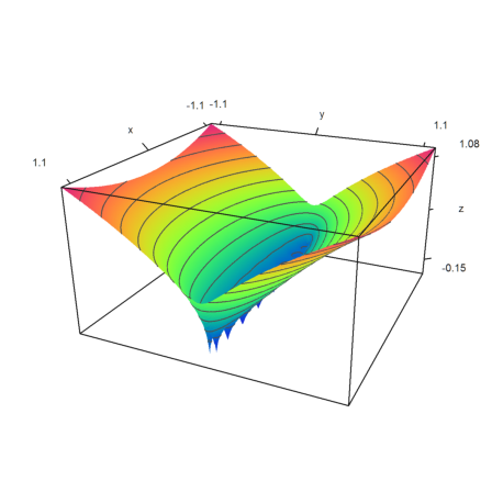
Here is the 3D view of the same function. We have to scale the values, so that the plot appears nicely in 3D.
>plot3d(x,y,log(w+0.2)/10,level=(0:10)/10,>hue,>spectral,zoom=3):
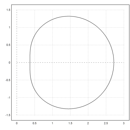
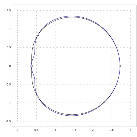
We construct an approximation to exp(z) on the unit circle by interpolation in 1,-1,i,-i, and compare this with the truncated power series.
First we plot the image of the unit circle.
>t=linspace(0,2pi,1000); z=exp(I*t); ...
 plot2d(exp(z),a=0,b=3,c=-1.5,d=1.5):
Then we add the interpolating polynomial.
>xp=[1,I,-1,-I]; yp=exp(xp); ...
 d=divdif(xp,yp); z1=evaldivdif(z,d,xp); ...
 plot2d(z1,color=4,>add); plot2d(exp(xp),>points,>add):
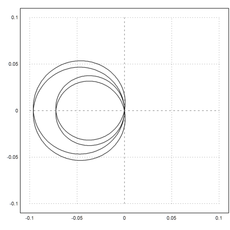
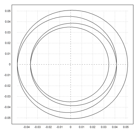
Plot the error function.
>plot2d(exp(z)-z1,r=0.1):
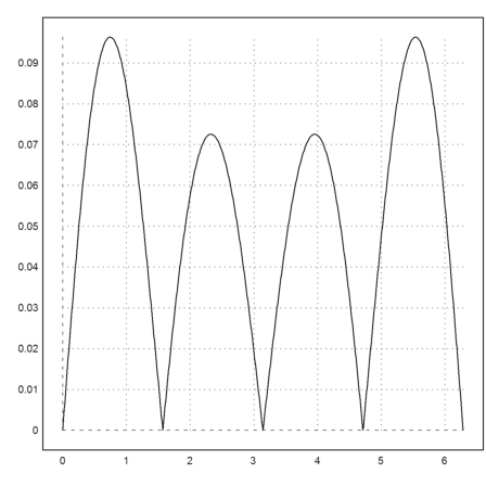
The absolute error.
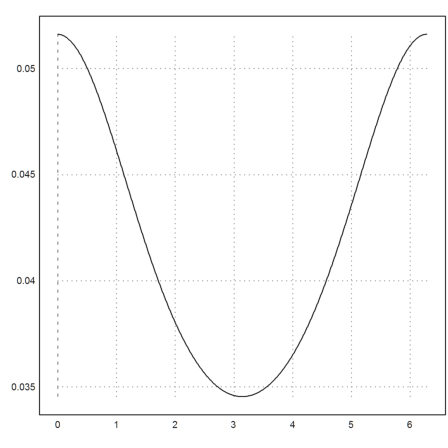
>plot2d(t,abs(exp(z)-z1)):
Plot the error of the truncated power series.
>z2=1+z+z^2/2+z^3/6; plot2d(exp(z)-z2):
Absolute error.
>plot2d(t,abs(exp(z)-z2)):