Euler can handle sound and graphics.
Sound can be created with the Euler matrix language, and analyzed with the Fast Fourier Transform (FFT). Euler can save sound in the wav file format, and play sounds in files.
Let us generate 5 seconds of sound. The default sampling rate is 44100 per second. First we need the time variable.
>t=soundsec(3);
Now generate a 440 Hz sound.
>s=sin(t*440)+sin(t*880)/2;
We can analyze it using FFT.
>shrinkwindow(>smaller); analyzesound(s):
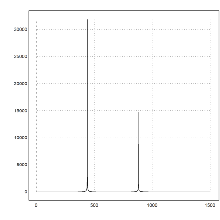
To play the sound, Euler saves the file in the user home directory. After playing the file, it is deleted.
>playwave(s);
We add some noise.
>s=s+normal(size(s)); analyzesound(s):
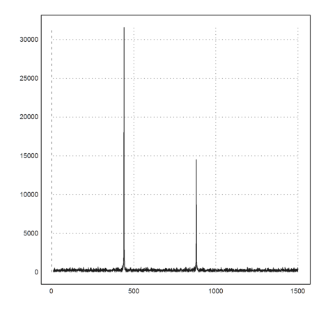
>playwave(s);
To fix this noise, we FFT the signal, and remove anything smaller than 0.1 times the maximal FFT result.
>f=fft(s); m=max(abs(f)); f=f*(abs(f)>0.1*m); sclear=re(ifft(f)); ...
 analyzesound(sclear):
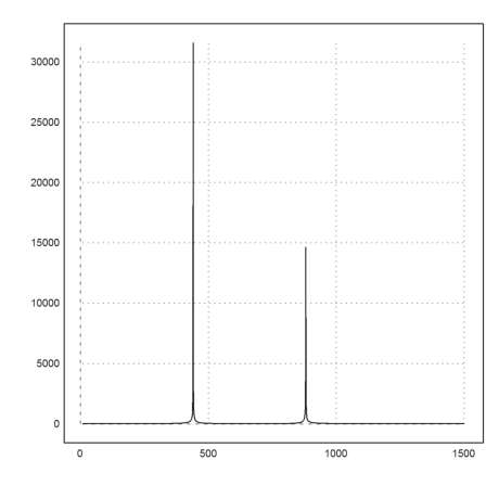
This clears the sound effectively.
>playwave(sclear);
We can also remove the sound with a filter. We use a simple filter, averaging over the 10 neighbors of each element.
>h=zeros(size(s)); h[1:10]=1/10*ones(1,10);
FFT can be used to fold a sound with the filter.
>s=fftfold(s,h);
The result is not perfect.
>playwave(re(s));
The sound utilities contain other functions to generate sounds. Let us add a few of them to one sound and play this sound.
>t=soundsec(0.6); ...
 s=sin(440*t)|soundtriangle(440*t)|soundpulse(440*t)|soundsaw(440*t); ...
 playwave(s);
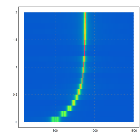
The mapsound function analyzes the sound in time windows. The time is vertical and the frequencies are horizontal.
You can see the changes in the frequencies. E.g., the triangle waves sound like a clarinet, because it uses odd frequencies.
>mapsound(s,fmax=4000):
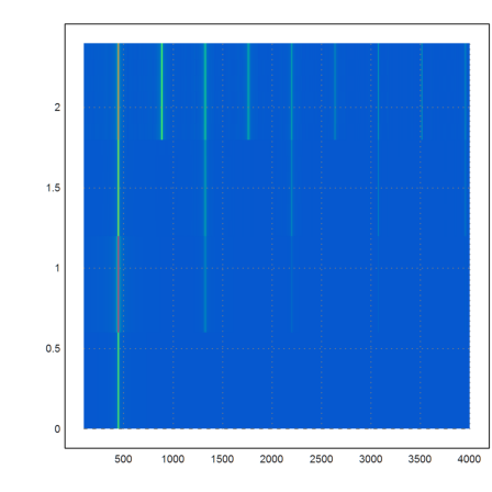
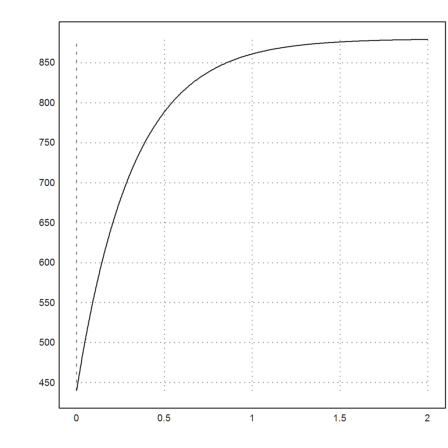
Let us change the frequency from 0 to 2 seconds, increasing from 440 to 880 Hz.
>function frequ(t) &= 880*(1-0.5*exp(-t/2)); ...
 plot2d("frequ(x*2*pi)",0,2):
To generate the correct sound, we need the integral of this frequency control function.
>function Frequ(t) &= integrate(frequ(t),t)
                                   - t/2
                         880 (1.0 E      + t)
Now, we can generate the sound.
>t=soundsec(2); s=sin(Frequ(t));
We can make a windowed FFT for this with the following function.
>mapsound(s):
And listen to the result.
>playwave(s);
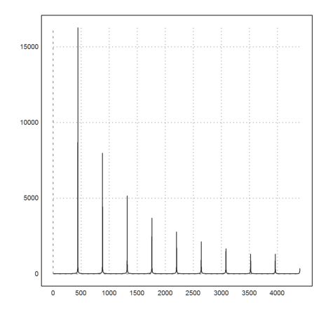
We can use the matrix language to generate frequencies. For an example, we generate
![]()
>t=soundsec(1); n=1:10; s=sum(sin(440*n*t')/n)'; playwave(s);
>analyzesound(s,fmax=4400):
To generate such a sum, we can also use Maxima and let it create the formula for us.
>cossum &= sum(sin(n*x)/n,n,1,10)
       sin(10 x)   sin(9 x)   sin(8 x)   sin(7 x)   sin(6 x)
       --------- + -------- + -------- + -------- + --------
          10          9          8          7          6
                    sin(5 x)   sin(4 x)   sin(3 x)   sin(2 x)
                  + -------- + -------- + -------- + -------- + sin(x)
                       5          4          3          2
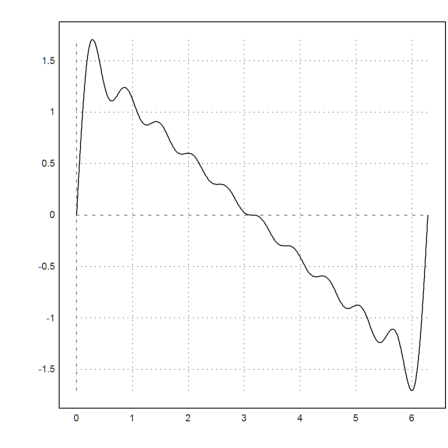
A single period of this wave looks like this.
>plot2d(cossum,0,2pi):
And we can evaluate this expression as usual in Euler.
>playwave(cossum(440*t));
For stereo sound, we need two rows of sound. Let us generate a 2 second sample of 220Hz.
>t=soundsec(4); s=sin(440*t)+sin(660*t)/2;
Now we fade the sound from left to right exponentially and put the two channels to a 2xn matrix v. We play it back and forth once.
>h=sin(t); v=((s*h)_(s*(1-h))); playwave(v);
For more examples on sound in Euler see the following notebooks.
Examples/Temperament in Musical Pitch
Examples/Sample Rates of Sound
Graphics can be stored in Euler in compact form, using one real number for each pixel, or in matrices of red-, green-, or blue-channel.
Let us create a colorful matrix.
>r=0:0.005:1; g=(0:0.005:1)'; M=rgb(r,g,0);
The matrix is plotted with the (0,0) corner in the lower left. The plot with "plotrgb" fills the current plot window.
>plotrgb(M);
The command "insrgb" inserts a rgb matrix into the text window. Note that the graphics is only 200x200.
>insrgb(M);

To save the file, we choose a location in the user home directory.
>file=userhome()|"test.png"
C:\Users\Rene\test.png
Save the file.
>savergb(M,file);
Load it back, and remove the file.
>M=loadrgb(file); fileremove(file);
Let us add some blue noise. To do this, we extract the red and green channels and set the blue channel to a random value, and reassemble this to a rgb image with the "rgb" function.
>insrgb(rgb(getred(M),getgreen(M),random(size(M))));
