In this notebook, we use Euler Math Toolbox (EMT) for the calculation of interest rates. We do that numerically and symbolically to show you how Euler can be used to solve real life problems.
Assume you have a seed capital of 5000 (say in dollars).
>K=5000
5000
Now we assume an interest rate of 3% per year. Let us add one simple rate and compute the result.
>K*1.03
5150
Euler would understand the following syntax too.
>K+K*3%
5150
But it is easier to use the factor
>q=1+3%, K*q
1.03
5150
For 10 years, we can simply multiply the factors and get the final value with compound interest rates.
>K*q^10
6719.58189672
For our purposes, we can set the format to 2 digits after the decimal dot.
>format(12,2); K*q^10
6719.58
Let us print that rounded to 2 digits in a complete sentence.
>"Starting from " + K + "$ you get " + round(K*q^10,2) + "$."
Starting from 5000$ you get 6719.58$.
What if we want to know the intermediate results from year 1 to year 9? For this, Euler's matrix language is a big help. You do not have to write a loop, but simply enter
>K*q^(0:10)
Real 1 x 11 matrix

    5000.00     5150.00     5304.50     5463.64     ...
How does this miracle work? First the expression 0:10 returns a vector of integers.
>short 0:10
[0, 1, 2, 3, 4, 5, 6, 7, 8, 9, 10]
Then all operators and functions in Euler can be applied to vectors element for element. So
>short q^(0:10)
[1,  1.03,  1.0609,  1.0927,  1.1255,  1.1593,  1.1941,  1.2299,
1.2668,  1.3048,  1.3439]
is a vector of factors q^0 to q^10. This is multiplied by K, and we get the vector of values.
>VK=K*q^(0:10);
We may wish to plot this.
>plot2d(VK);
If you have your plot window hidden, press the tabulator key to see the plot.
We can do better. In the following line of commands, we first plot the line of growth as above, but with the proper time scale. Then we add the data points on a second plot with the >points and >add parameters.
>plot2d(0:10,VK); plot2d(0:10,VK,>points,>add):
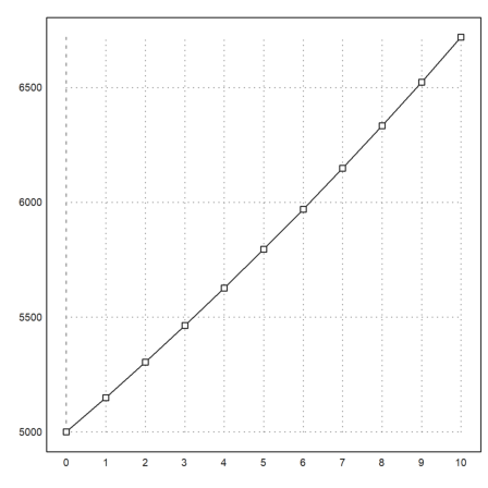
We inserted the plot into the command window with the colon. Inserted images are saved and also exported to HTML.
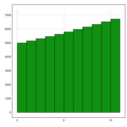
We might use a bar plot instead. For this, we add the parameter >bar (or bar=1) to the arguments for the plot2d function.
>plot2d(0:11,VK,>bar):
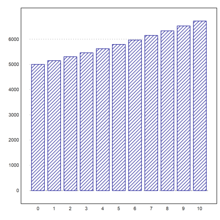
There are many more routines to plot in Euler. Here is the columns plot from the statistics package.
>columnsplot(VK,0:10,color=blue,style="/"):
Of course, the realistic way to compute these interest rates would be to round to the nearest cent after each year. Let us add a function for this.
>function oneyear (K) := round(K*q,2)
Let us compare the two results, with and without rounding.
>longest oneyear(1234.57), longest 1234.57*q
                1271.61
              1271.6071
Now there is no simple formula for the n-th year, and we must loop over the years. Euler provides many solutions for this.
The easiest way is the function iterate, which iterates a given function a number of times.
>VKr=iterate("oneyear",5000,10)
Real 1 x 11 matrix

    5000.00     5150.00     5304.50     5463.64     ...
We can print that in a friendly way, using our format with fixed decimal places.
>VKr'
    5000.00
    5150.00
    5304.50
    5463.64
    5627.55
    5796.38
    5970.27
    6149.38
    6333.86
    6523.88
    6719.60
To get a specific element of the vector, we use indices in square brackets.
>VKr[2], VKr[1:3]
    5150.00
    5000.00     5150.00     5304.50
Surprisingly, we can also use a vector of indices. Remember that 1:3 produced the vector [1,2,3].
Let us compare the last element of the rounded values with the full values.
>VKr[-1], VK[-1]
    6719.60
    6719.58
The difference is very small.
By the way, the iterate function can also be used to iterate until convergence occurs. Convergence is detected by comparing the new value with the old in relation to the internal epsilon. For an example, we iterate the well known recursive sequence
![]()
>longest iterate("(x+2/x)/2",1)
1.414213562373095
Here, we used an expression instead of a function in iterate(). By convention, an expression in x works like a function.
Now we take a more advanced function, which adds a certain rate of money each year.
>function onepay (K) := K*q+R
We do not have to specify q or R for the definition of the function. Only if we run the command, we have to define these values. We select R=200.
>R=200; iterate("onepay",5000,10)
Real 1 x 11 matrix

    5000.00     5350.00     5710.50     6081.82     ...
What if we remove the same amount each year?
>R=-200; iterate("onepay",5000,10)
Real 1 x 11 matrix

    5000.00     4950.00     4898.50     4845.45     ...
We see that the money decreases. Obviously, if we get only 150 of interest in the first year, but remove 200, we lose money each year.
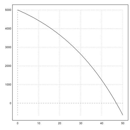
How can we determine the number of years the money will last? We would have to write a loop for this. The easiest way is to iterate long enough.
>VKR=iterate("onepay",5000,50)
Real 1 x 51 matrix

    5000.00     4950.00     4898.50     4845.45     ...
Using the matrix language, we can determine the first negative value in the following way.
>min(nonzeros(VKR<0))
48.00
The reason for this is that nonzeros(VKR<0) returns a vector of indices i, where VKR[i]<0, and min computes the minimal index.
Since vectors always start with index 1, the answer is 47 years.
The function iterate() has one more trick. It can take an end condition as an argument. Then it will return the value and the number of iterations.
>{x,n}=iterate("onepay",5000,till="x<0"); x, n,
     -19.83
      47.00
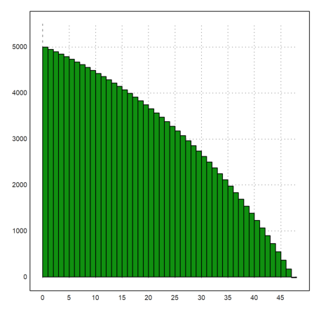
Here is the decline in graphical form.
>plot2d(0:47,VKR[1:48],>bar):
Let us try to answer a more ambiguous question. Assume we know that the value is 0 after 50 years. What would be the interest rate?
This is a question, which can only be answered numerically. Below, we will derive the necessary formulas. Then you will see that there is no easy formula for the interest rate. But for now, we aim for a numerical solution.
The first step is to define a function which does the iteration n times. We add all parameters to this function.
>function f(K,R,P,n) := iterate("x*(1+P/100)+R",K,n;P,R)[-1]
The iteration is just as above
![]()
But we do longer use the global value of R in our expression. Functions like iterate() have a special trick in Euler. You can pass the values of variables in the expression as semicolon parameters. In this case P and R.
Moreover, we are only interested in the last value. So we take the index [-1].
Let us try a test.
>f(5000,-200,3,47)
-19.83
Now we can solve our problem.
>solve("f(5000,-200,x,50)",3)
3.15
The solve routine solves expression=0 for the variable x. The answer is 3.15% per year. We take the start value of 3% for the algorithm. The solve() function always needs a start value.
We can use the same function to solve the following question: How much can we remove per year so that the seed capital is exhausted after 20 years assuming an interest rate of 3% per year.
>solve("f(5000,x,3,20)",-200)
-336.08
Note that you cannot solve for the number of years, since our function assumes n to be an integer value. The iterate function will not work for non-integer numbers of iterations.
But there is the function intbisect(), which uses a bisection algorithm and evaluates only on integer values. At the end, it interpolations between the two integer values, where the function changes its sign. In our case, we get between 20 and 21 years.
>intbisect("f(5000,-330,3,x)",10,30)
20.50
We can use the symbolic part of Euler to study the problem. First we define our function onepay() symbolically.
>function op(K) &= K*q+R
R + q K
We can now iterate this.
>&op(op(op(op(K)))), &expand(%)
                   q (q (q (R + q K) + R) + R) + R


                      3      2                4
                     q  R + q  R + q R + R + q  K
We see a pattern. After n periods we have
![]()
The formula is the formula for the geometric sum, which is known to Maxima.
>&sum(q^k,k,0,n-1); & % = ev(%,simpsum)
                          n - 1
                          ====        n
                          \      k   q  - 1
                           >    q  = ------
                          /          q - 1
                          ====
                          k = 0
This is a bit tricky. The sum is evaluated with the flag "simpsum" to reduce it to the quotient.
Let us make a function for this.
>function fs(K,R,P,n) &= (1+P/100)^n*K + ((1+P/100)^n-1)/(P/100)*R
                       P      n
                100 ((--- + 1)  - 1) R
                      100                    P      n
                ---------------------- + K (--- + 1)
                          P                 100
The function does the same as our function f before. But it is more effective.
>longest f(5000,-200,3,47), longest fs(5000,-200,3,47)
     -19.82504734650985
     -19.82504734652684
We can now use it to ask for the time n. When is our capital exhausted? Our initial guess is 30 years.
>solve("fs(5000,-330,3,x)",30)
20.51
This answer says that it will be negative after 21 years.
We can plot f as continuous function of the time, whatever sense this may make.
>plot2d("fs(5000,-200,3,x)",0,50):
We can also use the symbolic side of Euler to compute formulas for the payments.
Assume we get a loan of K, and pay n payments of R (starting after the first year) leaving a residual debt of Kn (at the time of the last payment). The formula for this is clearly
>equ &= fs(K,R,P,n)=Kn
                     P      n
              100 ((--- + 1)  - 1) R
                    100                    P      n
              ---------------------- + K (--- + 1)  = Kn
                        P                 100
Usually this formula is given in terms of
![]()
>equ &= (equ with P=100*i)
                          n
                  ((i + 1)  - 1) R          n
                  ---------------- + (i + 1)  K = Kn
                         i
We can solve for the rate R symbolically.
>&solve(equ,R)
                                           n
                           i Kn - i (i + 1)  K
                      [R = -------------------]
                                     n
                              (i + 1)  - 1
To plot the yearly rate depending on the interest rate, we define a function R.
>&solve(equ,R); function R(K,Kn,i,n) &= R with %
                                         n
                         i Kn - i (i + 1)  K
                         -------------------
                                   n
                            (i + 1)  - 1
Now we can plot this function, assuming full paying back in 10 years for interest rates of 0 to 10%.
>plot2d("R(5000,0,x/100,10)",0,10):
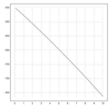
As you can see from the formula, this function returns a floating point error for i=0. Euler plots it nevertheless.
Of course, we have the following limit.
>&limit(R(5000,0,x,10),x,0)
- 500
Clearly, without interest we have to pay back 10 rates of 500.
The equation can also be solved for n. It looks nicer, if we apply some simplification to it.
>fn &= solve(equ,n) | ratsimp
                                  R + i Kn
                              log(--------)
                                  R + i K
                         [n = -------------]
                               log(i + 1)
How long can we take 200 from a seed capital of 5000 until it is reduced to half? This depends on the interest rate in the following way.
>plot2d(&fn with [K=5000,Kn=2500,R=-200,i=x/100],0,4):
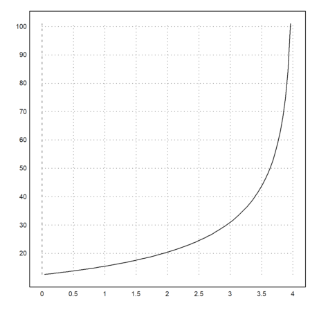
Clearly, for P=0% we get 12.5 years, and for P=4% we get infinite payments.
Euler has a library of functions for interest rates. The functions are stored in a so-called Euler file, which must be loaded.
>load interest
Computes interest rates for investments.
The file is in the path of Euler directories.
>path
C:\euler\util;C:\euler\docs\Programs\Examples;C:\Users\reneg\Euler;
But if you put your Euler file in the same directory as the current directory, it will be found.
If you look at the User Menu now, you find some patterns there, which help you to use the library. An example is the first function, which computes an interest rate depending on a vector of payments.
Another way to get help is to open the help window with F1 and to enter "interest.e" there.
Let us assume we invest 1000 and get two returns of 600. This makes the payments of the following vector.
>v=[1000,-600,-600]; columnsplot(v,0:2):
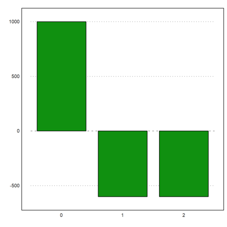
Then the first function of the menu computes the interest rate for this investment.
>rate(v)
13.07
This is computed by solving the following equation for i.
>eq &= 1000-600/(1+i)-600/(1+i)^2
                         600      600
                      - ----- - -------- + 1000
                        i + 1          2
                                (i + 1)
This equation discounts the payments to the current date. After replacing
![]()
we get a polynomial.
>eq &= eq with i=1/x-1
                              2
                       - 600 x  - 600 x + 1000
Since is is only a polynomial of degree 2, we can solve it exactly.
>&solve(eq,x)
                     - sqrt(69) - 3      sqrt(69) - 3
                [x = --------------, x = ------------]
                           6                  6
We can immediately evaluate this in Euler.
>&solve(eq,x)()
-1.88 0.88
Extracting the second element of this vector, we can compute the interest rate.
>&solve(eq,x)()[2], (1/%-1)*100
       0.88
      13.07
Let us compute an example with 4 returns.
>v=[1000,-400,-200,-200,-400]; columnsplot(v,0:4):

The numerical result is no problem.
>rate(v)
7.76
Now let us generate the symbolic polynomial.
>p &= sum(@v[k]*x^(k-1),k,1,5)
                     4        3        2
              - 400 x  - 200 x  - 200 x  - 400 x + 1000
We did not define the vector v symbolically. It is a numerical variable. But we can use it in a symbolic formula with @v nevertheless to form the polynomial as a sum.
The polynomial has two real roots.
>plot2d(p,-2,2):
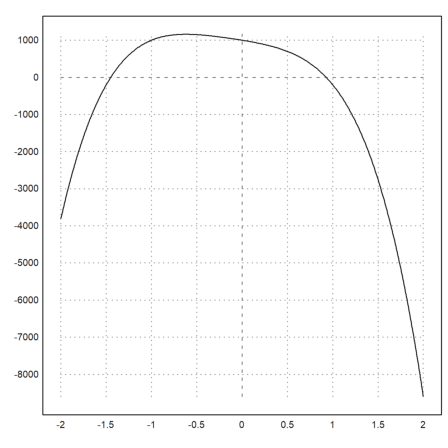
The symbolic solutions are not nice, to say the least. The vector of solutions in string form has almost 1700 characters. The Latex formula is still ugly. We do not print it.
>&solve(p); strlen(&%)
1693.00
Here is the expression of the root we are interested in.
>&x with solve(p)[2]
                   5 sqrt(12487)   785 1/6
        sqrt((171 (------------- + ---)   )
                          3/2      432
                      16 3
              5 sqrt(12487)   785 2/3       5 sqrt(12487)   785 1/3
/(8 sqrt(144 (------------- + ---)    - 39 (------------- + ---)
                     3/2      432                  3/2      432
                 16 3                          16 3
            5 sqrt(12487)   785 1/3               125
 - 500)) - (------------- + ---)    + ---------------------------
                   3/2      432           5 sqrt(12487)   785 1/3
               16 3                   36 (------------- + ---)
                                                 3/2      432
                                             16 3
   13                5 sqrt(12487)   785 2/3
 - --)/2 - sqrt(144 (------------- + ---)
   24                       3/2      432
                        16 3
       5 sqrt(12487)   785 1/3             5 sqrt(12487)   785 1/6
 - 39 (------------- + ---)    - 500)/(24 (------------- + ---)   )
              3/2      432                        3/2      432
          16 3                                16 3
   1
 - -
   8
This is not nice. And for polynomials of degree 5 or larger, it is impossible to get such a formula.
Maxima can evaluate the solutions numerically.
>&float(solve(p))
        [x = - 1.450269257619282, x = 0.9280281675050956,
x = 0.01112054505709326 - 1.362858124003226 I,
x = 1.362858124003226 I + 0.01112054505709326]
But it expresses the solutions in a way, which cannot be evaluated by Euler, since it uses roots of negative numbers. To force Euler to make everything complex, we set a special flag for one evaluation.
>longest complex:&"solve(p)"()
Complex 1 x 4 matrix

                          -1.450269257619282+0i     ...
Let us check the result with a numerical solution.
>&x with solve(p)[2]; longest %(), longest solve(p,1)
     0.9280281675050956
      0.928028167505094
In fact, this agrees with the result of the rate() function.
>Psol=(1/solve(p,1)-1)*100
7.76
We can simulate the states of this investment with the correct interest rate. The last value must be 0.
>simrate(v,Psol)
1000.00 677.55 530.10 371.21 0.00
Another function of this library answers the rate problem above. We need a seed value, the yearly returns, and the start and end year.
>investment(1000,-300,1,6)
15.22
The following is the same, but much easier to remember.
>v=1000|dup(-300,5)', rate(v)
Real 1 x 6 matrix

    1000.00     -300.00     -300.00     -300.00     ...
      15.24
Let us assume a normal distributed interest rate of 3% with 0.5% standard deviation. This is a realistic scenario if we cannot fix the interest rate.
In Euler we can simulate this. There is the sequence function for iterations like this. First we generate random factors. For this we combine a vector of 10 0-1-distributed values with the matrix language of Euler.
>n=10; q=1+(3+normal(1,10)*0.5)/100; long q
[1.03289701886,  1.02442643843,  1.03283878097,  1.02842697888,
1.03132001167,  1.02018595729,  1.02750695004,  1.0209736152,
1.0282450712,  1.03309482541]
The sequence function is an easy way to do complicate iterations. To make sure, we pass the variable q to the function.
>K=5000; R=-200; sequence("x[n-1]*q[n-1]+R",5000,11;q)
Real 1 x 11 matrix

    5000.00     4964.49     4885.75     4846.19     ...
It is more transparent to do the programming in handwork. Euler has a fairly sophisticated, but easy to learn programming language.
>function onerun (K,R,n,mean=3,dev=0.5) ...
 res=zeros(1,n);
 q=1+(mean+normal(1,10)*dev)/100;
 x=K;
 for i=1 to n;
   x=x*q[i]+R; res[i]=x;
 end;
 return K|res
 endfunction
Let us test.
>onerun(5000,-200,10)
Real 1 x 11 matrix

    5000.00     4923.95     4894.56     4805.65     ...
Now we can do a Monte-Carlo simulation. We could write another function. But we can also put the loop into a single command line.
>n=10000; VR=zeros(1,n);  ...
   for i=1 to n; VR[i]=onerun(5000,-200,10)[-1]; end;
The function plot2d can plot distributions automatically.
>plot2d(VR,>distribution):
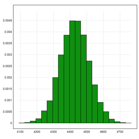
The mean value of this agrees with the undisturbed value.
>mean(VR), fs(5000,-200,3,10)
    4426.90
    4426.81