by R. Grothmann
Games of strategy can be analyzed in Euler
In this notebook, we provide examples for all three methods. You will see that games in math are a fascinating subject.
We start the following simple game:
Throw a dice, and decide, if you want to accept, or to try another throw. If you try again and throw the same or something less you lose and get nothing. If you decide to stop you get the current value. You can repeat that as often as you want.
What is the best strategy, and what is the average win?
You might notice that this is similar to Jeopardy, where you have a chance to answer each question correctly and promote, or fall back to nothing. The probabilities may be harder to nail down, but the idea is the same.
The solution is to work back from the 6 to the 1 and compute the expected win for each throw. The value of a 6 is just 6. For any lower number, we decide to throw again if the expected value of higher numbers is better than the value we have.
Let us make a function for this.
>function value (n) ...
 v=1:n;
 for i=n-1 to 1 step -1;
   v[i]=max(v[i],sum(v[i+1:n])/n);
 end
 return v
 endfunction
>value(6)
[3.5, 3, 3, 4, 5, 6]
The result is, that we keep 3 to 6, and try again with 1 and 2. The 2 has value 3, since
![]()
and the 1 has a better value (!) since
![]()
Note that we take the value 3 for the number 2 to compute the value of 1. I.e., if we throw a 2 after the 1, we throw again.
The expected win is a bit more than 4.
>fraction mean(value(6))
49/12
What, if we play the same game with a deck of 1000 cards?
>v=value(1000); plot2d(v):
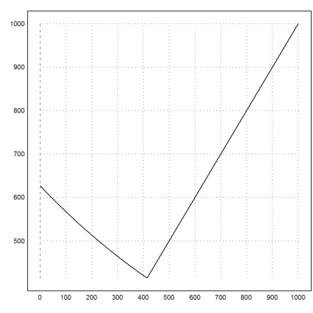
It is clear that v(x)=x for x large enough. The turning point is at 414, where we are better off to try again.
>min(v)
414.595
The expected win is about 627.
>mean(value(1000))
627.093265271
Let us explain this graph. We play the game in the interval [0,1], choosing points there at random. If we get x, and choose to continue, our expected win is the average of v(t) for t>=x.
![]()
First of all, the turning point s is easy to compute, since v(t)=t for t>=s.
>&integrate(t,t,x,1), &solve(%=x,x)
                                     2
                                1   x
                                - - --
                                2   2


                 [x = - sqrt(2) - 1, x = sqrt(2) - 1]
The value of s is the second solution. It explains the turning point at 414 we observed in the discrete case for n=1000.
>s=sqrt(2)-1
0.414213562373
Left of s, we can differentiate the equation which defines v and get
![]()
with the solutions
![]()
We determine lambda, such that the two branches fit.
>lambda=s/exp(-s)
0.626779782174
Now we can make a function of that.
>function v(x) := max(lambda*(exp(-x)),x);
The function looks as expected from the case n=1000.
>plot2d("v",0,1):
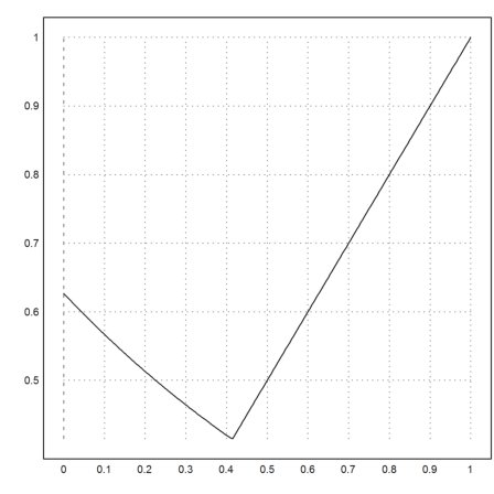
The expected win is just lambda as computed above.
>romberg("v",0,s)+romberg("v",s,1)
0.626779782174
We can get the same result in Maxima using symbolic analysis.
>s &= sqrt(2)-1; lambda &= s/exp(-s),
                                     sqrt(2) - 1
                      (sqrt(2) - 1) E
>&integrate(lambda*exp(-x),x,0,s)+integrate(x,x,s,1) | ratsimp
                                     sqrt(2) - 1
                      (sqrt(2) - 1) E
It is also possible to compute the discrete results exactly. We seek a discrete function with
![]()
It is clear, that v(k)=k for large i.
>&assume(k>0,n>0); sk &= sum(i,i,k+1,n)/n | simpsum | factor
                         (n - k) (n + k + 1)
                         -------------------
                                 2 n
We compute the turning value k0. So we search the largest value k, where v(k)>k. In this case, v(k) becomes the sum on the right side of its equation.
>&solve(sk=k,k); k0 &= k with %[2]
                            2
                    sqrt(8 n  + 8 n + 1) - 2 n - 1
                    ------------------------------
                                  2
The fraction k0/n has the known limit.
>&limit(k0/n,n,inf)
sqrt(2) - 1
For smaller values than k0, we get
![]()
Thus
![]()
![]()
So it is no surprise, that the exponential function appears. In fact, we get the same result in the limit.
>&(1+1/n)^k0*k0, &limit(%/n,n,inf) | ratsimp
                        2
                sqrt(8 n  + 8 n + 1) - 2 n - 1
                ------------------------------
          1                   2
        ((- + 1)
          n
                                            2
                                   (sqrt(8 n  + 8 n + 1) - 2 n - 1))/2


                                     sqrt(2) - 1
                      (sqrt(2) - 1) E
The rules of this game are quite simple. You probably know it: Each player selects secretly rock, paper or scissors, and both show their selection with hand signs at the same time. The win matrix for this game is the following.
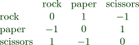
Our selection is one of the columns, and the selection of the opponent is one of the rows. The outcomes are in the table, seen from our side.
I.e., rock wins against scissors, scissors win against paper, and paper wins against rock (paper wraps the rock).
>A := [0,1,-1;-1,0,1;1,-1,0]; shortest A
        0         1        -1
       -1         0         1
        1        -1         0
We develop a worst case tactics. So we select probabilities
![]()
for each item. With these we compute the minimal expected win under all possible selections of the opponent. This is the worst case for our selection of probabilities. We get
![]()
for all rows i, where h is the minimal win.
The best strategy with the least worst case outcome maximizes h under the above conditions, and the additional condition
![]()
This can be translated into a problem of linear programming.
>M := A|-1; ...
 M := M_[1,1,1,0]; ...
 shortest M
        0         1        -1        -1
       -1         0         1        -1
        1        -1         0        -1
        1         1         1         0
The variables are p1,p2,p3,h. The first three rows are the inequalities,
![]()
and the last one is the equality
![]()
The right hand side is 0 for the inequalities, and 1 for the equality.
>b := zeros(rows(A),1)_1
            0
            0
            0
            1
The equation type is 1 (>=) or 0 (=).
>eq := [1,1,1,0]'
            1
            1
            1
            0
The target is to maximize h, the last variable.
>c := zeros(1,cols(A))|1
[0, 0, 0, 1]
Now we can start the Simplex algorithm.
>fraction simplex(M,b,c,eq=eq,restrict=[1,1,1,0],max=1,>check)
      1/3
      1/3
      1/3
        0
The result is, that we have to select each item with the same probability. The worst outcome is 0.
I have put this all into the function game(A) contained in the file game.e.
>load games.e;
This function computes the optimal strategy p, and the worst case result.
>{p,res}=game(A); fraction p,
[1/3, 1/3, 1/3]
>res
0
There is a modification of the game, with an additional item "well", which wins against scissors and rock (fall into well). The matrix for this is the following.
>A1 := [0,1,-1,1;-1,0,1,-1;1,-1,0,1;-1,1,-1,0]; shortest A1
        0         1        -1         1
       -1         0         1        -1
        1        -1         0         1
       -1         1        -1         0
The old optimal probabilities can no longer be used, since the opponent can beat them by selecting "well" all the time.
In fact, we get a different solution. We play paper, scissors, and well with equal probability.
>{p,res}=game(A1); fraction p
[0, 1/3, 1/3, 1/3]
The worst case is still 0. The game is fair. It must be fair, since it is absolutely symmetric. The game matrix for the opponent is -A'.
>res
0
The most simple Poker game goes like this: Both players get a random number from 1 to n.
In the latter case the player with the larger number gets the staked amount (wins 2$). With the same numbers, the outcome is 0.
The first player has three tactics:
1. pass all the time
2. hold with 1, pass with 2
3. pass with 1, hold with 2
4. hold with 1 and 2
2. is clearly inferior to 4., so we do cancel it from the list. The tactics remaining can be labelled
1. --
3. -+
4. ++
The second player has a similar list. The outcome is somewhat difficult to compute, since it depends on the probabilities of 1 and 2.
E.g., if player 1 selects -+ and player 2 selects -+, player 1 will loose 1$ when he gets a 1, and win 1/2$ on average when he gets a 2, since the other player in this case will pass with 1 and hold with 2. Thus the expected win of tactics -+ against -+ is
![]()
for the first player. This is of course an expected loss of 1/4.
E.g., let us compute -+ against ++. For 1, the first player gets -1$. For a 2 he wins 2$ with chance 1/2, yielding 1$ on average. The total average is 0$.
We fill out the matrix carefully.
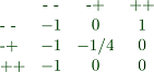
>B1 := [-1,0,1;-1,-1/4,0;-1,0,0]; fraction B1
       -1         0         1
       -1      -1/4         0
       -1         0         0
The following optimization says, that the first player has to select ++ all the time. If he doesn't the second player can punish him with -+.
>game(B1)
[0, 0, 1]
We can compute the optimal strategy of the second player using the transposed matrix with reverted outcomes. He can select -+ all the time. But it is clear that he can also select ++.
>game(-B1')
[0, 0, 1]
We can try to expand this method to more than 2 values. Let us assume the players get 1 to n randomly with equal probability 1/n.
We consider only the tactic i: "Pass with less than i" for both players. E.g., i=1 means: "Pass never". One can see easily that this is the best tactic, which passes for i-1 card values.
First we build a matrix, which shows the outcome, if player 1 selects j, and player 2 selects i, for each card value 1 to n of player 1, and 1 to n of player 2.
>function T (i,j,n) ...
   in=1:n; jn=in';
   H=2*(jn<in)-2*(jn>in);
   if j>1 then H[1:n,1:j-1]=-1; endif;
   if i>1 then H[1:i-1,j:n]=1; endif;
   return H
 endfunction
In the following example, player 2 does not pass with cards greater or equal 3, and player 1 does not pass with cards greater or equal 2. Here n=4.
Consequently, player 1 will lose 1$ with a 1, and player 2 will lose 1$, if player 1 has 2 or more, and he has less than 3. In all other cases, we can just compare cards for a loss or win of 2$.
>shortest T(3,2,4)
       -1         1         1         1
       -1         1         1         1
       -1        -2         0         2
       -1        -2        -2         0
Now we can compute the expected value for strategies i and j.
>function map expect (i,j,n) := totalsum(T(i,j,n))/n^2
The matrix A(n) in the following function is our game matrix.
>function A(n) := expect((1:n)',1:n,n)
The case n=2 is the lower right 2x2 matrix of above, but with columns and rows inverted, since ++ is now i=1 resp. j=1.
>A(2)
            0             0
            0         -0.25
Here is the 5x5 case.
>shortest A(5)
        0      0.12      0.08     -0.12     -0.48
    -0.12     -0.04     -0.04      -0.2     -0.52
    -0.08     -0.12     -0.16     -0.28     -0.56
     0.12     -0.04      -0.2     -0.36      -0.6
     0.48       0.2     -0.08     -0.36     -0.64
Now we can compute the optimal strategy for player 1.
>{p,res}=game(A(5)); fraction p'
      2/3
      1/3
        0
        0
        0
This result shows that a random bluff is a good move. Bidding with card value 1 looks unnatural at first sight. But we have to do it with probability 2/3.
The game is no longer fair. It is a loss for player 1.
>fraction res
-7/75
If we forbid player 1 to bid with card 1, he loses more.
>M5=A(5); M5[:,1]=-1; ...
 {p,res}=game(M5); fracprint(p'), res
        0
        1
        0
        0
        0
-0.12
Let us look at the strategy for player 2. It turns out, that this player has to be more reasonable.
>{p,res}=game(-A(5)'); fracprint(p'), res
        0
      1/3
      2/3
        0
        0
0.0933333333333
Let us try to disallow holding with 1 or 2 for player 2. The result is worse.
>M5=-A(5)'; M5[:,1:2]=-1;
>{p,res}=game(M5); fracprint(p'), res
        0
        0
        1
        0
        0
0.08
The case n=100 takes about 5 seconds on my computer. This is due to the generation of the the matrix A(n), which could be improved using a more direct formula. The Simplex algorithm is rather quick.
>A100=A(100); {p,res}=game(A100);
The result is: Never pass in 66% of the games, and pass in 0.34% of the games, if you have less than 34. You will lose 0.11 on average.
>nonzeros(p), fraction p[nonzeros(p)]', res
[1,  34]
    65/99
    34/99
-0.111066666667
Let us check, if this is indeed the worst case for the strategy v.
>min((A100.p')')
-0.111066666667
The strategy for the second player is the following.
>{p,res}=game(-A100'); ...
 nonzeros(p), fraction p[nonzeros(p)]', res
[34,  35]
      2/3
      1/3
0.111066666667
In the continuous case, both players get a number between 0 and 1 with equal distribution in [0,1]. From our experiments, we think that we should bid always in 2/3 of the games, and bid with 1/3 or better in the rest 1/3 of the games.
We like to compute the worst case loss for this strategy. The equivalent of our matrix is a function
![]()
If the first player has strategy y ("pass with less than y"), and the second player strategy x ("pass with less than x"), then for y>x
Other cases balance out. Carefully computing the chances for y>x and y<=x leads to the following function.
>function f(x,y) ...
   if y>x then return -y+(1-y)*x+2*(y-x)*(1-y)
   else return -y+(1-y)*x-2*(x-y)*(1-x)
 endfunction
>plot3d("f",a=0,b=1,c=0,d=1,angle=120°,contour=true):
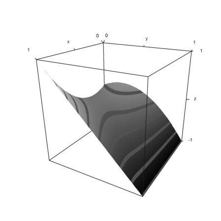
The result is as expected. For our strategy, the worst case occurs for x=1/3.
>xopt := fmin("2/3*f(x,0)+1/3*f(x,1/3)",0,1)
0.333333336154
And it has the value -1/9.
>2/3*f(xopt,0)+1/3*f(xopt,1/3)
-0.111111111111
We claim that the optimal strategies are
For the first player:
For the second player:
We already checked the outcome of the strategy of the first player. It is an average loss of -1/9.
Let us check the outcome for the second player.
>yopt := fmax("f(1/3,x)",0,1)
0.0896659076396
Indeed, the outcome is 1/9.
>fraction -f(1/3,yopt)
1/9
This proves that both strategies are optimal. The proof is rather obvious. But it is also a case of a duality relation in optimization.
Let us simulate the game with both players playing the optimal strategy. The following function gets a random number for both players and a random number for the first player, so that he can select his strategy.
>function map onegame (x,y,xrand) ...
 if xrand<1/3 and x<1/3 then return -1; endif
 if y<1/3 then return 1; endif;
 if x>y then return 2;
   else return -2;
 endif
 endfunction
The simulation should be close to -1/9 as expected.
>n=100000; sum(onegame(random(1,n),random(1,n),random(1,n))/n)
-0.10889
I recently found the following game in a beautiful book by Peter Winkler (Mathematische Rätsel für Liebhaber). The game starts with a row of coins of various values. The players in turn can take a coin from either end of the row. The problem is to show that the first player cannot lose if the game starts with an even number of coins. I will present the solution at the end of the notebook.
The following is just a programming lesson, and has nothing to do with numerical math or symbolic solutions. We will compute the optimal strategy for this game.
So we start by defining a simple recursive function for the optimal value a player can achieve. The vector x contains the values of the coins.
>function f(x) ...
 n=cols(x);
 if n>1 then
  return max(x[1]-f(x[2:n]),x[n]-f(x[1:n-1]))
 else
  return x[1]
 endif
 endfunction
It should not be too difficult to see, why this works. Let us test some examples, where the optimal strategy is clear. E.g., if the coins are increasing from the left to right, it is obviously(?) best to take the coins at the large end.
E.g., the win for the first player is n (1 at each take), if the coins are 1 to 2n.
>f(1:10)
5
In the next example, we have to take ones, until the second player is forced to uncover the 10. So the win is 10-1=9.
>f([1,10,1,1,1,1,1,1])
9
If we want to know the optimal move, we need to return it too. So I change the code a bit.
>function fi(x) ...
 n=cols(x);
 if n>1 then
  e=extrema([x[1]-(fi(x[2:n])),x[n]-(fi(x[1:n-1]))]);
  return {e[3],e[4]}
 else
  return {x[1],1}
 endif
 endfunction
>side=["left","right"];
1 means left and, and 2 means right end.
>{a,i}=fi(1:10); a, side[i],
5
right
For a challenge, let us simulate an optimal game.
>function simulate (x) ...
 n=cols(x);
 if mod(n,2)==0 then "A takes:" else "B takes:" endif;
 if n==1 then x[1], return x[1]; endif
 {a,i}=fi(x);
 if i==1 then x[1]|" from the left", simulate(x[2:n]);
 else x[n]|" from the right", simulate(x[1:n-1]);
 endif
 return a
 endfunction
>v=simulate([1,10,20,30,10,1]); "Result:", v,
1 from the right
1 from the left
10 from the left
20 from the left
30 from the left
10
Result:
10
>simulate(1:5);
5 from the right
4 from the right
3 from the right
2 from the right
1
The recursion in the example above works for a small number n of coins. However, it generates 2^n function calls.
To avoid this in a recursive algorithm, we can add some memory for function results. In fact, there are only n^2 possible coin positions during the game.
So we add a matrix to denote the optimal value for the position x[i],...,x[j] in A[i,j] and the optimal move in I[i,j]. We set up the matrices once, and use the fact that Euler passes matrices by reference. Assigning to a submatrix will in fact change the matrix.
>function fifastrek (x,i,j,I,A) ...
 if I[i,j] then return A[i,j]; endif;
 if i==j then A[i,j]=x[i]; I[i,j]=i; return x[i], endif;
 a1=x[i]-fifastrek(x,i+1,j,I,A); a2=x[j]-fifastrek(x,i,j-1,I,A);
 if a1>a2 then I[i,j]=i; A[i,j]=a1; return a1;
 else I[i,j]=j; A[i,j]=a2; return a2;
 endif;
 endfunction
Instead of global matrices, we write a main function.
>function fifast (x) ...
 n=cols(x); I=zeros(n,n); A=zeros(n,n);
 return fifastrek(x,1,n,I,A);
 endfunction
Now we can solve 100 coins, which would be unthinkable with the simple recursion above.
>fifast(1:100)
50
How about the proof that the first player can always win at an even number of coins?
This is very simple with a trick. Number the coins from left to right. If you think about it, you see that the starting player can either take all the even coins, or all the odd coins. So he simply chooses, which is better.
>function g(x) ...
 n=cols(x);
 return abs(sum(x[2:2:n])-sum(x[1:2:n]))
 endfunction
>g([1,10,20,30,10,1])
10
However, this is not the optimal strategy! In the following example the odd coins 4+6 yield a win of 1. But it is better to take the 7 first, and then either the 4 for a win of 3, or the 6 for a win of 7.
>h=[4,2,6,7]; g(h), fifast(h),
1
3