by R. Grothmann
We want to study the catenary using measurements of a real chain, comparing the experiment to the theory.
First we read the data of the experiment from a file. I got these measurements by hanging a necklace at the computer screen, and marking some points with Euler and its mouse() function.
>P=getmatrix(24,2,"kette.dat")';
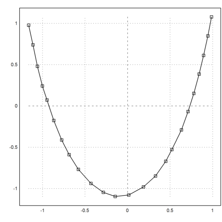
Let us plot these data.
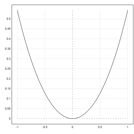
>plot2d(P[1],P[2]); ...
 plot2d(P[1],P[2],add=1,points=1,style="[]"):
Now we try to fit a parabola to these data.
>p=polyfit(P[1],P[2],2); ...
 y=polyval(p,P[1]); ...
 plot2d(P[1],y,color=10,add=1):
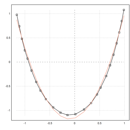
This does not look very good. The catenary is not a parabola.
Let us imagine the necklace as mass points connected by massless cords of fixed length. In each cord, there is some force vector (x,y). The forces from the two cords adjacent to a mass point, and the gravitational force of the point must add to 0.
So, if we study the triangle of forces in each mass point of the necklace, we see that the y-component of the force in the cords, increases by a fixed amount from cord to cord. The x-component remains equal.
>ky=-1:0.01:1; kx=ones(size(ky));
Now we have the forces in each cord. The cords go into the directions of the forces. To get the cords, we normalize the forces, since all forces are of equal length.
>ds=sqrt(kx*kx+ky*ky)*100;
Now we compute the cumulative sum of the cords, and get the catenary.
>X=0|cumsum(kx/ds); Y=0|cumsum(ky/ds);
We normalize the catenary, so that its deepest point is in y=0, and symmetric to the y-axis.
>X=X-(X[1]+X[cols(X)])/2; Y=Y-min(Y);
And plot it.
>plot2d(X,Y):
If we look into a physics book, the catenary with deepest point in (0,0) should be a function of the kind y=a*cosh(x/a)-a. We can try to determine the constant a for our simulated curve, by interpolating the above curve in X[1], using the bisection method to solve for a. The result is just a=1.
>a=solve("x*cosh(X[1]/x)-x-Y[1]",1)
1.00002390404
The following is the maximal deviation of the cosh curve to our simulation.
>y1=a*cosh(X/a)-a; max(abs(Y-y1))
1.24997272464e-005
Now we want to fit a cosh function to our measured data. However, we face the problem that our computer screen, and our Euler window were not exactly square in x- and y-direction. So we need additional parameters of freedom. We use functions of the type
![]()
and minimize the sum of squared differences of y and the measured values.
>function f(x) := sum((x[1]*cosh((P[1]-x[2])/x[3])-x[4]-P[2])^2)
We compute the minimum with the Nelder-Mead method.
>x=neldermin("f",[1,1,1,1],0.001,eps=0.0001);
Let us plot the measured data again.
>plot2d(P[1],P[2]); ...
 plot2d(P[1],P[2],add=1,points=1,style="[]");
We add the fit to the plot.
>plot2d(P[1],x[1]*cosh((P[1]-x[2])/x[3])-x[4],add=1,color=10):
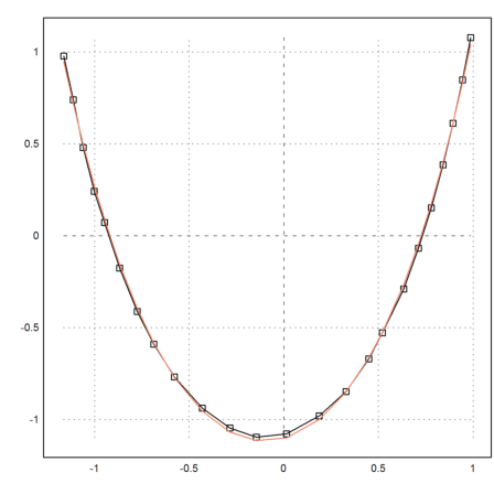
This looks like a satisfying result. There are still some glitches in the middle, which might be problems with the approximation of the necklace by a catenary, or with the measurement.
In the sequel, we try to hang a catenary of given length between two given points. There is no exact solution for this. We need to use a numerical method to solve the problem.
So we set up a general catenary function.
>function k (x,a,b,c) &= a*(cosh((x-b)/a))-c
                                 x - b
                          a cosh(-----) - c
                                   a
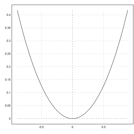
Test it.
>plot2d("k",-1,1;1,0,1):
Since we want to use the length of this catenary, we compute the length element ds of this curve with Maxima.
>function kd (x,a,b,c) &= sqrt(1+diff(a*cosh((x-b)/a),x)^2)
                                 2 x - b
                        sqrt(sinh (-----) + 1)
                                     a
And integrate it with a Gauß quadrature.
>gauss("kd",-1,1;1,0,1)
2.35040238729
Let us make a function for this.
>function kl (x1,x2,a,b,c) := gauss("kd",x1,x2;a,b,c)
We have to solve the interpolation condition k(x1)=y1, k(x2)=y2, as well as the length condition k1(x1,x2)=length. So we define a function for this error.
>function res (v,x1,y1,x2,y2,length) ...
 return (k(x1,v[1],v[2],v[3])-y1)^2 ..
 + (k(x2,v[1],v[2],v[3])-y2)^2 ..
 + (kl(x1,x2,v[1],v[2],v[3])-length)^2
 endfunction
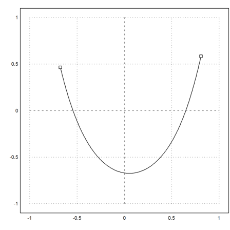
A test with y(-1)=0.8, y(1)=0.5, and length 3.
>v=neldermin("res",[1,0,0];-1,0.8,1,0.5,3);
Plot it.
>plot2d("k",-1,1;v[1],v[2],v[3]);
Also the length is correct.
>kl(-1,1,v[1],v[2],v[3])
2.99999991995
The following function waits for two mouse clicks and compute the catenary.
>function test (length) ...
 clg; setplot(-1,1,-1,1); xplot(); title("Two clicks!");
 m1=mouse(); hold on; mark(m1[1],m1[2]); hold off;
 m2=mouse(); hold on; mark(m2[1],m2[2]); hold off;
 setplot();
 v=neldermin("res",[1,0,0];m1[1],m1[2],m2[1],m2[2],length);
 t=linspace(m1[1],m2[1],300); s=map("k",t;v[1],v[2],v[3]);
 plot2d(t,s,a=-1,b=1,c=-1,d=1);
 plot2d([m1[1],m2[1]],[m1[2],m2[2]],points=1,add=1);
 return v
 endfunction
Now click two times in the upper region of the plot window.
>v=test(3):
Finally, we try to derive the catenary function.
In the simulation, we saw that the force has constant x-coordinate, and an x-coordinate increasing with the length. We get the force of the tye (d,c+a*s(x)), where s(x) is the length. Since the force and the catenary have the same slope, we get
![]()
differentiating to x, we get
![]()
Since the curve length is the integral of sqrt(1+y'^2), we get
![]()
Let us solve this in Maxima.
>eq &= 'diff(y,x,2) = k*sqrt(1+'diff(y,x)^2)
                        2
                       d y           dy 2
                       --- = k sqrt((--)  + 1)
                         2           dx
                       dx
>&ode2(eq,y,x)
                         cosh(k x + %k1 k)
                     y = ----------------- + %k2
                                 k
We get the well known formula, the same formula we used above in the form
![]()
Note that a catenary is different from the curve of a rope bridge (a bridge hanging at parallel ropes in equal distances).
We approximate this as a street hanging at a weightless rope. In this case, the force does not accumulate with the length of the rope, but with the length of the street! So we get the much easier differential equation
![]()
with a parabola as a solution.