by R. Grothmann
Gauss integration is defined in Euler in the gauss() function. We like to show, how to derive a Gauss formula.
First we need the Legendre polynomials. These polynomials are orthogonal on [-1,1]. We simply use Gram-Schmidt. To ease the compuation, we define the scalar product in Maxima.
>function sp(f,g) &&= integrate(f*g,x,-1,1)
integrate(f g, x, - 1, 1)
Then we need p0 to p4.
>p0 &= 1;
>p1 &= x;
>p2 &= x^2-sp(x^2,p0)/sp(p0,p0)*p0
                                 2   1
                                x  - -
                                     3
>p3 &= x^3-sp(x^3,p1)/sp(p1,p1)*p1
                                3   3 x
                               x  - ---
                                     5
>p4 &= x^4-sp(x^4,p2)/sp(p2,p2)*p2-sp(x^4,p0)/sp(p0,p0)*p0 | ratsimp
                              4       2
                          35 x  - 30 x  + 3
                          -----------------
                                 35
There is a function legendre(), which computes these polynomials using a recursion formula.
>fracprint(legendre(4)*8)
[3, 0, -30, 0, 35]
This agrees with the result of Maxima.
>&expand(legendre_p(4,x)*8)
                              4       2
                          35 x  - 30 x  + 3
We need the zeros of p4. Maxima can provide these zeros in exact form.
>&solve(p4), xnode=%()
              sqrt(2 sqrt(30) + 15)      sqrt(2 sqrt(30) + 15)
       [x = - ---------------------, x = ---------------------,
                    sqrt(35)                   sqrt(35)
                     sqrt(15 - 2 sqrt(30))      sqrt(15 - 2 sqrt(30))
               x = - ---------------------, x = ---------------------]
                           sqrt(35)                   sqrt(35)

[-0.861136,  0.861136,  -0.339981,  0.339981]
Now we need to define the coefficients of the formula. We solve the equation
![]()
for
![]()
The matrix language of Euler lets us easily define a linear system for this.
>A=xnode^((0:3)'); b=(2*[1,0,1/3,0])'; ...
 alpha=(A\b)'
[0.347855, 0.347855, 0.652145, 0.652145]
These values can also be obtained by the Christoffel function in the following way.
For this, the polynomials must be normalized with respect to the L2-norm.
>function C4(x) &= 1/sum(legendre_p(n,x)^2/ ...
   integrate(legendre_p(n,x)^2,x,-1,1),n,0,3) | ratsimp
                                  8
                     ---------------------------
                          6        4       2
                     175 x  - 165 x  + 45 x  + 9
Indeed, we get exactly the same values.
>C4(xnode)
[0.347855, 0.347855, 0.652145, 0.652145]
We can test this for the interval [-1,1].
>function map gauss5test (f) := sum(f(xnode)*alpha); ...
 fraction gauss5test(["1","x","x^2","x^3","x^4","x^5","x^6","x^7","x^8"])
[2, 0, 2/3, 0, 2/5, 0, 2/7, 0, 258/1225]
The result is exact for polynomials of degree 7.
We define a function for this integration using the Euler matrix language. The matrix X in the following function, contains all knots in all subintervals. Knots with equal coefficients are collected in each row.
>function gauss5test (f,a:number,b:number,n=1,xn=xnode,al=alpha) ...
 h=(b-a)/n;
 if n>1 then x=linspace(a+h/2,b-h/2,n-1); else x=a+h/2; endif;
 X=x-(h/2*xn)';
 return sum(al.f(X))*h/2
 endfunction
Test.
>fracprint(gauss5test("x^6",0,1))
1/7
Let us test some more functions. The n=10 subintervals are 40 function evaluations.
>longestformat; gauss5test("exp(x)",0,1,10)-(E-1)
4.440892098500626e-016
The function is already defined in Euler.
>longestformat; gauss5("exp(x)",0,1,10)-(E-1)
4.440892098500626e-016
Note that
![]()
The Simpson method is not so good, but takes half as many function evaluations.
>simpson("exp(x)",0,1,10)-(E-1)
5.964481175624314e-008
The Gauss algorithm with 10 knots gets the same result with only 10 evaluations.
>gauss("exp(x)",0,1)-(E-1)
2.220446049250313e-016
Here is a test with the Gauss distribution.
>gauss5("exp(-x^2/2)",0,10,n=10)/sqrt(2*pi)
0.5000000000028569
>gauss("exp(-x^2/2)",0,10,n=10)/sqrt(2*pi)
0.5000000000000001
In the following, we compute the Legendre polynimals explicitely using the symbolic functions of Euler and Maxima.
The Legendre satisfy the following recursion formula.
![]()
To program such a recursion in Maxima, we define the following purely symbolic function with a function body containing a block of statements.
>function L(x,n) &&= block ( ...
   if n=0 then 1 ...
   else if n=1 then x ...
   else ((2*n-1)*x*L(x,n-1)-(n-1)*L(x,n-2))/n )
       block(if n = 0 then 1 else (if n = 1 then x
                       (2 n - 1) x L(x, n - 1) - (n - 1) L(x, n - 2)
                  else ---------------------------------------------))
                                             n
>&L(x,2)
                                  2
                               3 x  - 1
                               --------
                                  2
Let us check the orthogonality.
>&integrate(L(x,2)*L(x,1),x,-1,1)
0
>&integrate(L(x,2)*L(x,0),x,-1,1)
0
>&integrate(L(x,3)*L(x,2),x,-1,1)
0
The norm of L(x,n) is 2/(2n+1).
>&integrate(L(x,2)*L(x,2),x,-1,1)
                                  2
                                  -
                                  5
The Legendre polynomials satisfy the following differential equation.
>eq &= -2*x*'diff(y,x)+(1-x^2)*'diff(y,x,2)+n*(n+1)*y=0
                         2
                     2  d y       dy
               (1 - x ) --- - 2 x -- + n (n + 1) y = 0
                          2       dx
                        dx
Test for n=3
>& eq | [n=3,y=L(x,3)], & % | nouns | ratsimp
                               2
                       5 x (3 x  - 1)
                   2   -------------- - 2 x
              2   d          2
        (1 - x ) (--- (--------------------))
                    2           3
                  dx
                         2
                 5 x (3 x  - 1)
                 -------------- - 2 x                2
             d         2                     5 x (3 x  - 1)
      - 2 x (-- (--------------------)) + 4 (-------------- - 2 x) = 0
             dx           3                        2


                                0 = 0
The main Maxima command ode2 cannot solve this.
>& eq | n=2, &ode2(%,y,x)
                             2
                         2  d y       dy
                   (1 - x ) --- - 2 x -- + 6 y = 0
                              2       dx
                            dx


                                false
The two term recursive definition can get ineffective. So we replace it with a loop.
>function L(x,n) &&= block( if n=0 then 1 else block([y:[1,x]], ...
  for i:2 thru n do y:[y[2],expand(((2*i-1)*x*y[2]-(i-1)*y[1])/i)], y[2]));
Test.
>& L(x,2) | ratsimp
                                  2
                               3 x  - 1
                               --------
                                  2
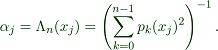
We can now use polynomials of high degree.
>plot2d(& L(x,20) | expand,-1,1):
For other weights, we could do just the same.
>function sp(f,g) &&= integrate(f*g*exp(-x),x,-1,1)
                                   - x
                    integrate(f g E   , x, - 1, 1)
Then we need p0 to p4.
>p0 &= 1;
>p1 &= x-sp(x,p0)/sp(p0,p0)|ratsimp
                              2
                            (E  - 1) x + 2
                            --------------
                                 2
                                E  - 1
>p2 &= x^2-sp(x^2,p1)/sp(p1,p1)*p1-sp(x^2,p0)/sp(p0,p0)*p0|ratsimp
          4      2       2         4       2           4      2
        (E  - 6 E  + 1) x  + (- 2 E  + 16 E  - 6) x - E  + 6 E  + 7
        -----------------------------------------------------------
                                4      2
                               E  - 6 E  + 1
If we continue like this, we get fairly complicated polynomials. We like to demonstrate, how to use numerical integration instead.
First, we define the function to integrate.
>function p(x,i) := x^i*exp(-x)
Then the integral.
>function map a(i) := gauss("p",-1,1,100;i)
A test.
>a(5)
-0.3242973696922066
>&integrate(x^5*exp(-x),x,-1,1), %()
                                       - 1
                           44 E - 326 E

-0.3242973696922178
It becomes obvious, that the result is not perfect. We either have to live with this, or to derive and use a recursion formula, or the exact symbolic method.
We need the 10-th orthogonal polynomial. To compute it, we use the Gram matrix.
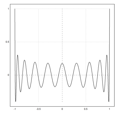
>A=a((0:10)+(0:9)')_1; b=zeros(10,1)_1;
>p=xlgs(A,b)';
Here is a plot of this polynomial.
>plot2d("polyval(p,x)",-1,1):
Let us test the orthogonality.
>for i=0 to 9; gauss("x^i*polyval(p,x)*exp(-x)",-1,1,100), end;
1.23084875625068e-014
-7.745415420146173e-014
-1.233568802661011e-014
3.418543226274551e-014
3.103073353827313e-016
-2.974398505273257e-014
-1.885935851930754e-014
6.401379426534959e-014
3.972544515562504e-014
-5.778488798569015e-014
Next we need the zeros.
>xn=sort(real(polysolve(p)))
[-0.9761983950159177,  -0.876341759205208,  -0.7038368925296208,
-0.4708613994245012,  -0.1948808338591103,  0.1018814014714706,
0.3935411401555917,  0.6524949822560991,  0.8523013113814679,
0.9712722677116907]
Then we need the coefficients, which make the integration exact for polynomials up to degree 9.
>M=xn^((0:9)'); b=a((0:9)');
>al=xlgs(M,b)'
[0.1616042035976784,  0.3308952772834531,  0.4148551396265188,
0.4128502394503031,  0.3529200553213233,  0.2698111100739772,
0.1888527845927684,  0.1216033541103824,  0.06925902427714205,
0.02775119895405546]
We can use the same code as above to define the Gauss integrator.
>function gauss10exp (f,a:number,b:number,n=1,xn=xn,al=al) ...
 h=(b-a)/n;
 if n>1 then x=linspace(a+h/2,b-h/2,n-1); else x=a+h/2; endif;
 X=x-(h/2*xn)';
 return sum(al.f(X))*h/2
 endfunction
Let us test with the integral of cos(x)*exp(-x).
>gauss10exp("cos(x)",-1,1)
1.933421496200713
This is the Gauß formula for one sub-interval.
>sum(cos(xn)*al)
1.933421496200713
The result is absolutely exact to all digits.
>&integrate(cos(x)*exp(-x),x,-1,1); %()
1.933421496200713