by R. Grothmann
We are going to demonstrate a direction search for the global minimization of a real valued function f. First we define a function, which evaluates another function at x into the direction v. The function vectorizes for t.
>function map %fveval (t; f, x, v) := f(x+t*v);
Using this, we can search from x into a direction of descent v.
First we establish a value t, such that f(x+tv) is increasing. We do this by doubling the steps t until the values increases. For simplicity, we assume that our function f is defined everywhere.
>function vmin (f,x,v,tstart,tmax=1,tmin=epsilon) ...
 ## Minimize f(x+t*v) assuming v is a direction of descent
 y=f(x);
 t=tstart;
 repeat
    ynew=f(x+t*v);
    while ynew<y;
    t=t*2;
    until t>tmax;
 end;
 t=fmin("%fveval",0,t;f,x,v);
 return {x+t*v,t};
 endfunction
For a gradient method, we need a function and its gradient. We take a very simple example for a first test.
>function f([x,y]) &= x^2+2*y^2
                                 2    2
                              2 y  + x
>function df([x,y]) &= gradient(f(x,y),[x,y])
[2 x, 4 y]
The function vmin minimizes f in a direction v, starting from the point x.
![]()
It returns the current step size t. This can be used as an initial step size in the next step.
>x0=[1,1]; {x1,t}=vmin("f",x0,-df(x0),0.1); x1,
[0.444444, -0.111111]
But it does not come close to the minimum in (0,0). Not even in two steps.
>{x2,t}=vmin("f",x1,-df(x1),t); x2,
[0.0740741, 0.0740741]
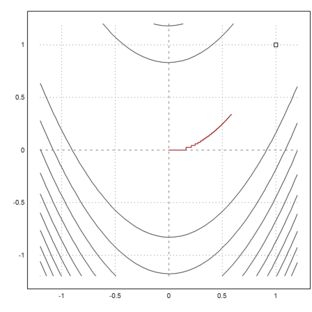
The reason becomes obvious if we look at the following plot, where the level lines of our iterations are shown.
>X=(x0_x1_x2)'; ...
   plot2d("f",r=2,level=[f(x0),f(x1),f(x2)],n=100);  ...
   plot2d(X[1],X[2],color=red,>add):
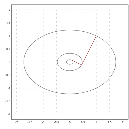
>X
            1      0.444444     0.0740741
            1     -0.111111     0.0740741
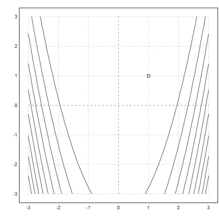
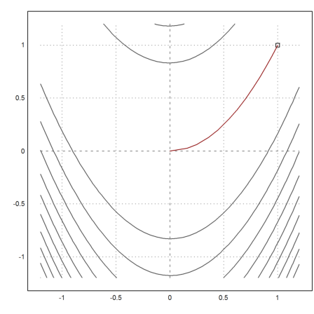
The situation improves, if we use a Newton direction
![]()
We can compute the general inverse Hessian with Maxima, and thus the direction of descent.
>function newtonvf([x,y]) &= -df(x,y).invert(hessian(f(x,y),[x,y]))
[ - x - y ]
This yields a very good result in just one step.
>x0=[1,1]; x1=vmin("f",x0,newtonvf(x0),0.1)
[1.03673e-012, 1.03673e-012]
Indeed, it is easy to see, that the Newton algorithm finishes in just one step for each linear function, and indeed, the gradient is a linear function. There is no need to compute the minimum of f(x+tv) in this case.
>x0+newtonvf(x0)
[0, 0]
Let us take another convex function, which is not a quadratic function.
>function f4([x,y]) &= x^2+y^4
                                4    2
                               y  + x
>function df4([x,y]) &= gradient(f4(x,y),[x,y])
                                      3
                             [2 x, 4 y ]
We take 100 steps of the gradient method.
>x=[1,1]; t=0.1; X=x;  ...
   loop 1 to 100; {x,t}=vmin("f4",x,-df4(x),t); X=X_x; end;  ...
   X=X';
And plot the result.
>plot2d("f",r=1.2,level=fmap(X[1,1:3],X[2,1:3]),n=100); ...
   plot2d(X[1],X[2],>add,color=red):
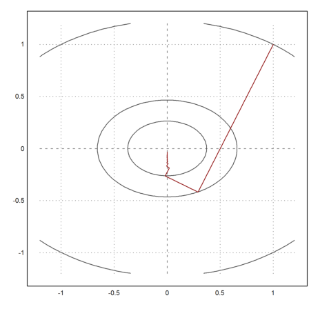
As we see, the result is not very good. Essentially the function takes a zig-zag-course in direction x, so that the y-value decreases only very slowly.
>X[:,-1]
-5.20883e-005
   -0.0333273
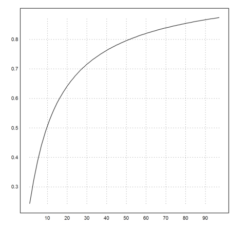
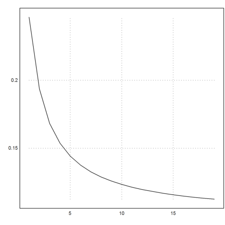
Here is the logarithmic descent
![]()
It is not very good.
>k=5:cols(X); plot2d(f4map(X[1,k],X[2,k])^(1/k)):
Let us try the Newton direction for this function.
>function newtonvf4([x,y]) &= -df4(x,y).invert(hessian(f4(x,y),[x,y]))
                             [        y ]
                             [ - x  - - ]
                             [        3 ]
Now we get good results after 20 iterations.
>x=[1,1]; t=0.1; X=x;  ...
   loop 1 to 20; {x,t}=vmin("f4",x,newtonvf4(x),t); X=X_x; end;  ...
   X=X';
>plot2d("f4",r=1.2,level=fmap(X[1,1:3],X[2,1:3]),n=100); ...
   plot2d(X[1],X[2],>add,color=red):
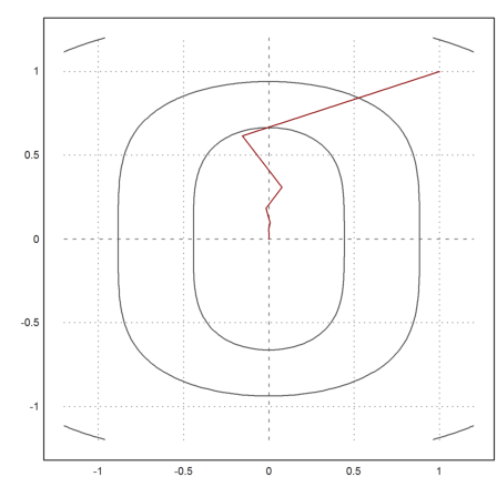
>X[:,-1]
  5.6658e-011
 9.61281e-006
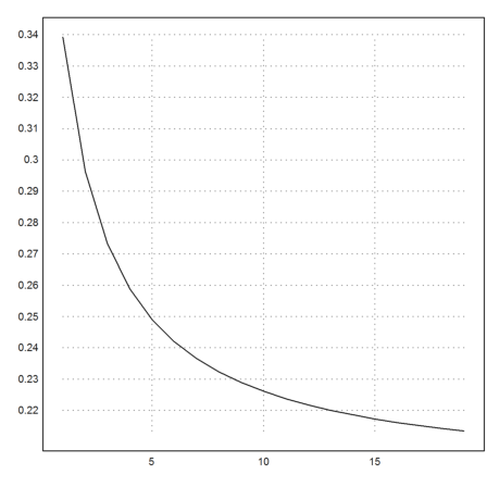
Here is the logarithmic descent.
>k=3:cols(X); plot2d(f4map(X[1,k],X[2,k])^(1/k)):
But the result is not so good, if we take the Newton algorithm itself.
>x=[1,1]; X=x;  ...
   loop 1 to 20; x=x+newtonvf4(x); X=X_x; end;  ...
   X=X';
This is in accordance with the observation that the Newton algorithm does not work well for the function f(y)=y^4.
>plot2d("f4",r=1.2,level=fmap(X[1,1:3],X[2,1:3])); ...
   plot2d(X[1],X[2],>add,color=red):
>X[:,-1]
            0
  0.000300729
>k=3:cols(X); plot2d(f4map(X[1,k],X[2,k])^(1/k)):
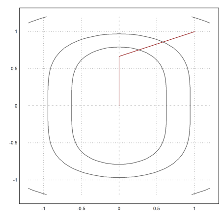
Now, we take another function, which is a well known test case.
>function fban([x,y]) &= 100*(y-x^2)^2+(1-x)^2;
The function
![]()
is not convex. It has a banana like behavior. The minimum is obviously in x=y=1.
>plot2d("fban",r=3,>contour,levels="thin"); plot2d(1,1,>points,>add):
>function dfban([x,y]) &= gradient(fban(x,y),[x,y])
                            2                         2
             [- 400 x (y - x ) - 2 (1 - x), 200 (y - x )]
We take 100 steps of the gradient method.
>x=[0,0]; t=0.1; X=x;  ...
   loop 1 to 100; {x,t}=vmin("fban",x,-dfban(x),t); X=X_x; end;  ...
   X=X';
And plot the result. The result does not even come close to the minimum. It takes a terrible step like zig-zag course.
>plot2d("fban",r=1.2,>contour,levels="thin"); plot2d(1,1,>points,>add); ...
   plot2d(X[1],X[2],>add,color=red):
Let us try the Newton method.
>function newtonvfban([x,y]) &= -dfban(x,y).invert(hessian(fban(x,y),[x,y]));
Now we get very good results after 20 iterations.
>x=[0,0]; t=0.1; X=x;  ...
   loop 1 to 20; {x,t}=vmin("fban",x,newtonvfban(x),t); X=X_x; end;  ...
   X=X';
>plot2d("fban",r=1.2,>contour,levels="thin"); plot2d(1,1,>points,>add); ...
   plot2d(X[1],X[2],>add,color=red):

>X[:,-1]
            1
            1
We implement Powell's method.
The idea is to start with a basis of directions, and minimize into each once. Then replace the best direction with the direction of the total descent into all directions.
For the implementation, we use the function brent(), which essentially works like vmin(), but searches into both directions.
>function minpowell (f$,x) ...
 history=x;
 n=cols(x); U=id(n);
 y=f$(x);
 d=zeros(1,n);
 repeat
    xold=x;
    ystart=y;
    loop 1 to n;
        yold=y;
        gamma=brentmin("%fv",0;f$,x,U[#]);
        x=x+gamma*U[#];
        y=f$(x);
        d[#]=yold-y;
    end;
    ex=extrema(d);
    U[ex[4]]=x-xold;
    y=f$(x); until y>=ystart;
    history=history_x;
 end;
 return history;
 endfunction
The method seems to perform very well for a method without derivatives. But one should be aware that each step costs n minimizations.
>v=minpowell("fban",[0,0])
            0             0
     0.161262     0.0260054
     0.249913     0.0624564
     0.357572      0.127858
     0.450678      0.203111
     0.541461      0.293181
     0.624952      0.390565
     0.702451      0.493437
     0.772832      0.597269
     0.835702      0.698397
     0.890175      0.792411
     0.935214      0.874625
     0.969359      0.939656
     0.990811      0.981706
     0.999069      0.998138
     0.999991      0.999983
            1             1
            1             1
            1             1
>X=v'; plot2d("fban",r=1.2,>contour,levels="thin");  ...
   plot2d(1,1,>points,>add); ...
   plot2d(X[1],X[2],>add,color=red):
The function is already implemented in Euler in powellmin().
>powellmin("fban",[0,0])
[1, 1]
The Nelder Mead method is another method for minimization without derivatives.
This demo shows the iterations for the Nelder-Mead minimization process.
We need to load helper functions for the demo.
>load "Nelder Mead Demo"
The Rosenbloom banana function, as needed by the Nelder method.
>function f([x,y]) &= 100*(y-x^2)^2+(1-x)^2
                                 2 2          2
                       100 (y - x )  + (1 - x)
The Minimum is in [1,1].
>&solve(gradient(f(x,y),[x,y]))
[[y = 1, x = 1]]
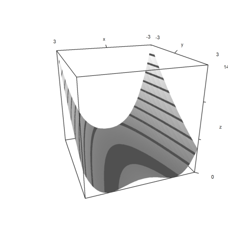
Plot in 3D, scaled
>plot3d("f",r=3,>contour,angle=160°,color=gray):
Plot the contour lines of the function in 2D. Add the minimum.
>plot2d("f",r=3,>contour,levels=(0:10:100)^2);  ...
 plot2d(1,1,>add,>points):
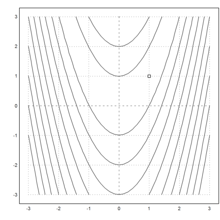
The Nelder-Mead method uses simplices. It moves one corner of the simplex, so that simplex moves towards a minimum.
Set the start simplex.
>s=[0,1;1,0;0,0];
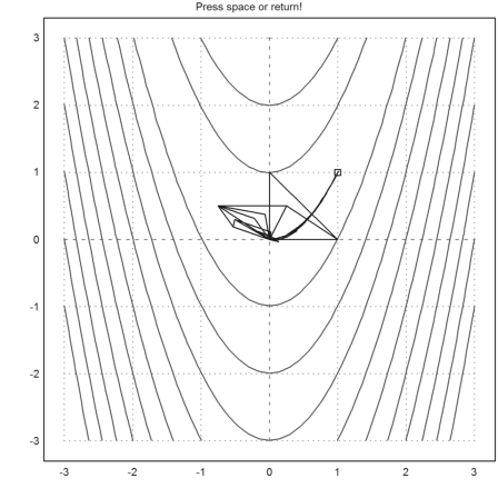
Show the iterations of the Nelder-Mead method.
Press Return to abort, and Space for the next step.
>nelderdemo(s,"f"):
Try the built-in function.
>nelder("f",[0,0])
[1, 1]