by R. Grothmann
The table of mortality contains the probability to die within one year depending on the current age and gender. I downloaded this table from the federal office for statistics (Bundesamt für Statistik) in Germany. Since the data are from a specific year (2009), it is clear that long term predictions are close to impossible. The medical treatment is certain to make enormous progress in short time periods.
The data are naked numbers in the data files
>load "mortality.e"; // load functions and data
The data are in the vectors pm and pf containing values
![]()
where qm[i] is the probability to die between the i-th and the (i+1)-th birthday (at the age of i) for males, resp. qf[i] for females. The probability to die before the first birthday is stored in qm0 and qf0.
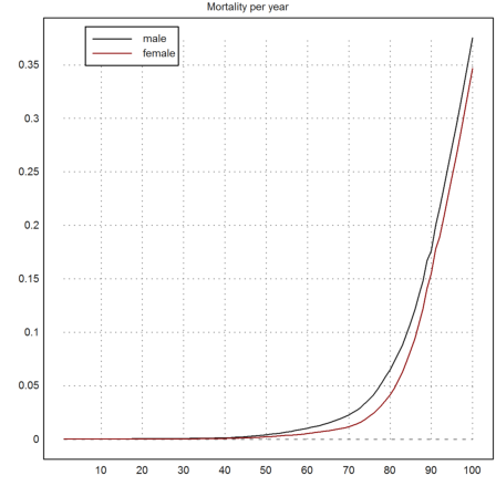
First we plot the probability do die at a given age. With the exception of very young children, this probability is an increasing function of age, smaller for females than for males.
>plot2d(1:100,qm); plot2d(1:100,qf,color=2,add=1);  ...
   title("Mortality per year"); ...
   labelbox(["male","female"],x=0.3,colors=[black,red]):
I do not know, if dead born children count to year 0, but probably they don't. Still the chance to die within the first year is exceptionally high. The probability to die decreases in the first years of the life.
>plot2d(0:20,qm0|qm[1:20],bar=1):
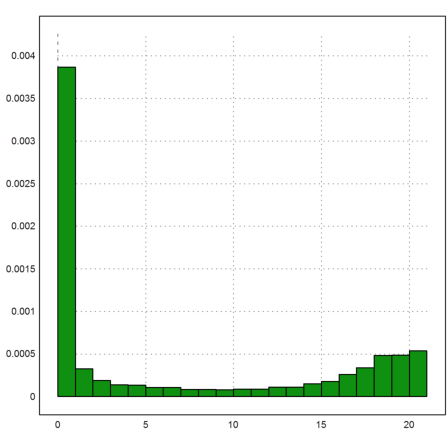
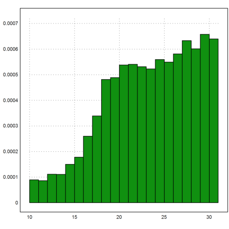
There is an interesting hump at the ages 18-22, which is due to the higher risks these ages are accepting.
>plot2d(10:30,qm[10:30],bar=1):
The probabilities are stored as fractions. We can also print them as percent. Here is the probability to die at the age of 53 for mail and female persons.
>print(qm[53]*100,unit="%"), print(qf[53]*100,unit="%"),
      0.55%
      0.30%
The probability to die within the two next years is more complicated. You either die now, or, if you survive, next year. E.g., the probability to die between the 53-th and 55-th birthday is
![]()
The answer is given as a fraction again.
>qm[53]+(1-qm[53])*qm[54]
0.0116784468641
We have for the chance to die at the age of m, if you are now n years old
![]()
Because you need to survive year n to m-1 and die in year m. Thus we get for the chance to die between the ages n to m
![]()
This can be easily computed using the Euler matrix language. The computation of q(n,m) uses the cumulative product.
>qm[53]+sum(cumprod(1-qm[53:62])*qm[54:63])
0.0940861514865
The computation has been coded into the function "ptodiewithin" contained in the mortality file. It takes two ages and a gender as parameters.
We see that the probability for males to die between 53 and 63 is double the probability for females.
>ptodiewithin(53,63,male), ptodiewithin(53,63,female)
0.0940861514865
0.0496752784217
The probability to die at the age of m, if you are now n, is contained in the function ptodiein(n,m,gender).
>ptodiein(53,63,male), ptodiein(53,63,female),
0.0116005288036
0.00644659115723
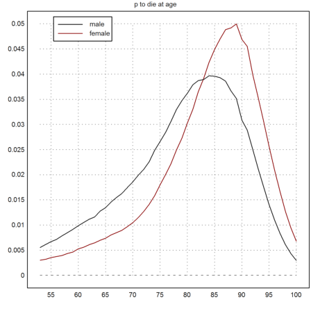
Now we can plot the probability to die at age 53 to 100 for males and females. We assume a starting age of 53.
>n=53;  ...
   plot2d(n:100,ptodiein(n,n:100,female),a=n,b=100,c=0,d=5%, ...
     color=red); ...
   plot2d(n:100,ptodiein(n,n:100,male),add=1); ...
   title("p to die at age"); ...
   labelbox(["male","female"],x=0.3,colors=[black,red]):
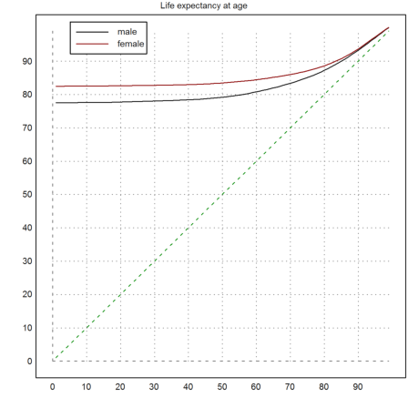
The life expectancy is the average dying age, given any current age.
To compute it, we have to multiply the probabilities to die at a given age times the age, and sum these.
![]()
The tables of mortality end at age 100, so we assume that all remaining people die at the age of 101.
In the example, the live expectancy of a 53 year old male is about 79.
>sum(ptodiein(53,53:100,male)*(53:100))+(1-ptodiewithin(53,100,male))*101
79.5558068927
This has been programmed in a function lifeexpect(n,gender).
Note that the expression above is not efficient, since it computes the cumulative sum for "ptodiein" several times. "lifeexpect" takes a more direct approach, of course.
>lifeexpect(53,male), lifeexpect(53,female),
79.5558068927
83.7027491609
Let us plot the life expectancy for each age. We add the current age in the plot to see the expected rest of life.
Mortality before the first birthday is not contained in these computations. So the average is under the condition that people get one year old.
>plot2d(1:99,lifeexpect(1:99,male),a=0,b=99,c=0,d=99); ...
   plot2d(1:99,lifeexpect(1:99,female),color=2,add=1); ...
   title("Life expectancy at age");  ...
   plot2d(1:99,1:99,color=green,style="--",add=1); ...
   labelbox(["male","female"],x=0.3,colors=[black,red]):
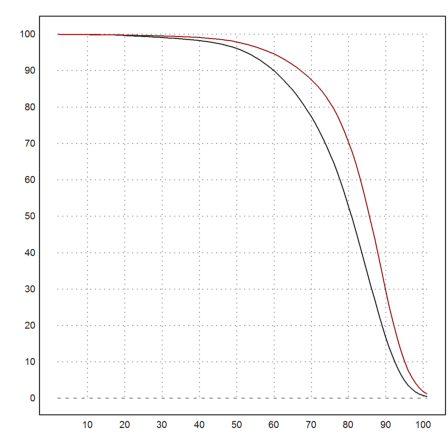
It might be interested to compute the median. This is the value such that half of the people are dead. Again, this is under the condition that they survived the first year.
We use the Euler language for this, computing the minimal year such that the probability to die before this year exceeds 0.5.
>min(nonzeros(ptodiewithin(1,1:100,male)>0.5))
80
For females this is 5 years more, as expected.
>min(nonzeros(ptodiewithin(1,1:100,female)>0.5))
85
Here is a plot of the surviving percentage.
>plot2d(2:101,(1-ptodiewithin(1,1:100,male))*100);  ...
 plot2d(2:101,(1-ptodiewithin(1,1:100,female))*100,color=red,add=true);  ...
   insimg;
Tables of mortality are used to compute insurance policies.
Let us assume, you are promised to get a life long pension of 1000, starting at your 65-th birthday, and you are now 53 years old. What would that be worth?
>P=1000; a0=53; a1=65;
We have to take into account the interest rate. Let us assume, we discount with 3% per anno.
>i=3%;
The value of this fond is the sum of the probabilities to survive to get the pension in each year from a1 to 100, discounted to the current date. Remember, that p(n,m) is the probability to die within age n to m. We assume that you have to survive year a1 to get your first pension payment.
![]()
It is far less than we expect.
>sum((1-ptodiewithin(a0,a1-1:100,male))*P/(1+i)^((a1-a0):(101-a0)))
8479.07972284
The computation is implemented in the function "pension". The comparison shows that a pension is worth a lot more for women.
>pension(53,65,3%,male)*P, pension(53,65,3%,female)*P,
8479.07972284
10207.8952139
Assume, I get ascending payments of 1000,1100,...,2000 starting at the end of the next year, under the condition that I still live. Let us store these values in a vector. The total amount of payments promised to me is the following.
>v=1000:100:2000; sum(v)
16500
What are these payments worth today?
To compute this, we have to compute the survival probability times the promised amount, discounted to the current date.
>sum(cumprod(1-qm[53:63])*v/(1+3%)^(1:11))
12946.9063204
There is a function for this.
>pensionv(53,v,3%,male), pensionv(53,v,3%,female),
12946.9063204
13261.2981285
If I live to get all the money without risk of dying, the value is a bit higher.
>sum(v/(1+3%)^(1:11))
13605.9243493
An important problem is a life insurance, which is payed in case of death only.
Assume, the life insurance promises an amount of K=100'000 in case of death during the next 10 years, starting with age 53. How high is the discounted risk for the insurance company? Note that the insurance does not pay the promised amount if we survive all 10 years. Remember that q(n,k) is the probability to die in age k, if you are now n years old.
![]()
To compute this, we have to multiply the probability to die in a year times the discounted sum, and add all these risks. As you see, in the formula discount a payment within the first year.
>K=100000; EK=sum(K*ptodiein(53,53:62,male)/(1+3%)^(1:10))
6906.32015735
How much would the company have to take for this risk?
To compute that, we assume the person pays the amount of R per year. We add the expected values of these payment, assuming pays in advance, discounted for today. The sum of these values is the expected discounted payment. Remember that p(n,k) is the probability to die at ages n to k.
![]()
To compute R, we divide the risk EK by the sum in brackets. The answer is the payment the company has to take each year (starting immediately).
>EK/(1+sum((1-ptodiewithin(53,53:61,male))/(1+3%)^(1:9)))
810.390016854
I packed the computation of the risk into a function, assuming K=1.
First a life insurance, which starts at age 53, and ends as soon as the person gets 63. The amount is not payed, if the person survives. The answer is the risk.
>EK=K*lifeinsurance(53,62,3%,male,pay=0)
6906.32015735
The computation of the discounted value of the payments is contained in another function. Dividing yields the rate R.
>EK/payments(53,62,3%,male)
810.390016854
Now a life insurance with the same parameters, but the sum will have to payed at the end, even if we survive. Now
![]()
Of course, this has a higher risk.
>EK=K*lifeinsurance(53,62,3%,male,pay=1)
75178.0066565
How much would the assurance company have to take for that each year? The value is much higher since we have to add the savings for the survival.
>EK/payments(53,62,3%,male)
8821.41353041
The same insurance would be cheaper for a woman, since she is expected to get the money later in case of death, and she is expected to pay her payments longer.
>K*lifeinsurance(53,63,3%,female)/payments(53,62,3%,female)
8410.31520292