by R. Grothmann
This is a translation of an introduction to Matlab by Cleve Moler. I found the file via Google on the following address.
http://www.mathworks.com/moler/intro.pdf
I try to do the same in Euler, so you can study the differences and similarities.
So the content of this notebook and the ideas are Moler's.
He begins by exploring the Golden Ratio, which is in fact the zero of the polynomial
![]()
>p=[-1,-1,1]
[-1, -1, 1]
The function of EMT for polynomial roots is polysolve(p).
>r=polysolve(p)
[ -0.618034+0i , 1.61803+0i ]
Of course, this can be solved exactly with Maxima. In Matlab with the symbolic toolbox, this would be a solution by Maple.
>&solve(1/x=x-1)
                       1 - sqrt(5)      sqrt(5) + 1
                  [x = -----------, x = -----------]
                            2                2
Maxima prints nicer than Matlab. However, it is a lot better to use Latex. EMT can display Latex formulas in comments or in the command line. In comments, we enter
maxima: solve(1/x=x-1)
and get
![]()
The polysolve() function returns complex roots. So let us make the second root real.
>real(r[2])
1.61803398875
Let us fix the value for phi.
>phi=(sqrt(5)+1)/2
1.61803398875
Maxima and Matlab can evaluate this to an arbitrary number of digits.
>&bfloat((sqrt(5)+1)/2)
1.6180339887498948482045868343656b0
The computation becomes arbitrarily slow, if you do this.
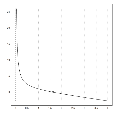
Functions like the following one line function can be done in Matlab too (a bit more ugly, however).
>function f(x) := 1/x-(x-1)
>plot2d("f",0,4);
>solve("f",1)
1.61803398875
>plot2d(phi,0,>points,>add):
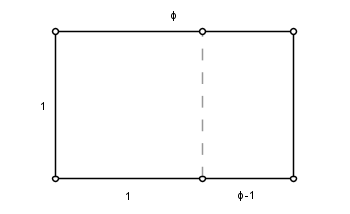
The following functions plots a sketch in Euler. The code is a translation from the Matlab code. In any case, it is not a good idea to use such programs for sketches.
>function plotgr ...
 phi = (1+sqrt(5))/2;
 x = [0,phi,phi,0,0];
 y = [0,0,1,1,0];
 u = [1,1];
 v = [0,1];
 plot2d(x,y,a=0,b=1.7,c=-0.7,d=1,<frame,<grid);
 plot2d(u,v,style="--",>add);
 text(latex("\phi"),toscreen([phi/2,1.1]));
 text(latex("\phi-1"),toscreen([(1+phi)/2,-.05]));
 ctext("1",toscreen([-.05,.5]));
 ctext("1",toscreen([.5,-.05]));
 endfunction
>plotgr; insimg(crop=0.7);
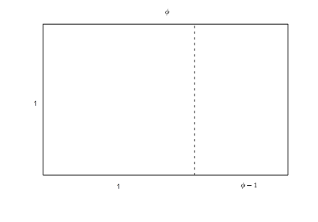
This is an abuse of Euler or Matlab. A graphical program like C.a.R. can do a nicer image with much less effort.
The next example in Moler's book is a continued fraction. Euler and Matlab can construct a string in the following way.
>p="1"; loop 1 to 6; p="1+1/("+p+")"; end; p,
1+1/(1+1/(1+1/(1+1/(1+1/(1+1/(1))))))
The string can be evaluated.
>p()
1.61538461538
This string is called a continued fraction. The fraction converges to the Golden Ratio phi.
>phi-p()
0.00264937336528
The following function is a direct translation of Matlab code. It determines the numerator and denominator of the continued fraction.
>function test(n) ...
   p = 1;
   q = 1;
   for k = 1:n
     s = p;
     p = p + q;
     q = s;
   end
   return{p,q}
 endfunction
>{p,q}=test(6); p+"/"+q
21/13
This is an approximation of phi.
Euler has the contfrac() function, which produces the continued fraction of a value. It also has the fracprint() function (or the "fraction" operator), which prints a value in fractional form (using continued fractions, by the way).
>contfrac((1+sqrt(5))/2,6), contfracval(%), fracprint(%)
[1,  1,  1,  1,  1,  1,  1]
1.61538461538
21/13
The following is a well known approximation of pi. It has been known since ancient times.
>contfrac(pi,3), api=contfracbest(pi,3), fraction api, api-pi
[3,  7,  15,  1]
3.14159292035
355/113
2.66764189405e-007
The following is a direct translation of the Matlab code.
>function fibonacci (n) ...
   f=zeros(1,n);
   f[1] = 1;
   f[2] = 2;
   for k = 3:n
     f[k] = f[k-1] + f[k-2];
   end
   return f
 endfunction
>fibonacci(12)
[1, 2, 3, 5, 8, 13, 21, 34, 55, 89, 144, 233]
Euler has the sequence command to produce this.
>sequence("x[n-2]+x[n-1]",[1,2],12)
[1, 2, 3, 5, 8, 13, 21, 34, 55, 89, 144, 233]
The following is the famous inefficient recursion.
>function fibnum (n) ...
   if n<=1 then return 1
   else return fibnum(n-1)+fibnum(n-2)
 endfunction
It works for small n. But the effort grows exponentially like 2^n.
>tic; fibnum(24), toc;
75025
Used 0.579 seconds
The quotients of successive Fibonacci numbers converges to phi.
>n=40; f=fibonacci(n);
>longestformat; (f[2:n]/f[1:n-1]-phi)', longformat;
Real 39 x 1 matrix

     0.3819660112501051
    -0.1180339887498949
    0.04863267791677184
   -0.01803398874989481
   0.006966011250105098
  -0.002649373365279484
   0.001013630297724166
 -0.0003869299263654646
  0.0001478294319232631
-5.646066000730698e-005
  2.15668056606777e-005
-8.237676933475768e-006
 3.146528619657474e-006
-1.201864648914253e-006
 4.590717870289751e-007
-1.753497695933248e-007
 6.697765919660981e-008
-2.558318845657936e-008
 9.771908393574336e-009
-3.732536946188247e-009
    ...
Indeed there is the famous formula for the Fibonacci numbers.
![]()
>n=1:40; 1/(2*phi-1)*(phi^(n+1)-(1-phi)^(n+1))
[1,  2,  3,  5,  8,  13,  21,  34,  55,  89,  144,  233,  377,  610,
987,  1597,  2584,  4181,  6765,  10946,  17711,  28657,  46368,
75025,  121393,  196418,  317811,  514229,  832040,  1346269,
2178309,  3524578,  5702887,  9227465,  14930352,  24157817,
39088169,  63245986,  102334155,  165580141]
This is a fractal generated by randomly selecting one of four transformations of the plane, and plotting the iterated points. The code is a translation of Matlab code.
>function fern (n) ...
 p = [ .85, .92, .99, 1.00];
 A1 = [ .85, .04; -.04, .85]; b1 = [0; 1.6];
 A2 = [ .20, -.26; .23, .22]; b2 = [0; 1.6];
 A3 = [-.15, .28; .26, .24]; b3 = [0; .44];
 A4 = [ 0, 0 ; 0, .16];
 x=[0.5;0.5];
 X=zeros(n,2);
 r=random(1,n);
 loop 1 to n;
   if r[#] < p[1]
     x = A1.x + b1;
   elseif r[#] < p[2]
     x = A2.x + b2;
   elseif r[#] < p[3]
     x = A3.x + b3;
   else
     x = A4.x;
   endif
   X[#]=x';
 end;
 return X;
 endfunction
We generate 100 thousand points.
>X=fern(100000)'; ...
 plot2d(X[1],X[2],a=-3,b=3,c=0,d=10, ...
   >points,<frame,<grid,style=".",color=green,>insimg);

It is clear, that neither Matlab nor Euler is good for type of iterations. In fact, a multi-core algorithm could generate this fractal much faster. Also it should really be done on the level of machine code.
>remvalue X;
Matlab had magic squares since the beginning. It is not clear why, since the program is essentially a numerical program like Euler.
>shortformat; A=magic(3)
        8         1         6
        3         5         7
        4         9         2
>sum(A)'
[15, 15, 15]
>sum(A')'
[15, 15, 15]
>sum(diag(A,0))
15
>sum(diag(flipy(A),0))
15
The sums must clearly be equal to the following.
>sum(1:9)/3
15
Like in Matlab, we can produce lots of permuted magic squares in the following way.
>for k=0:3; rot(A,k), "", end;
        8         1         6
        3         5         7
        4         9         2

        6         7         2
        1         5         9
        8         3         4

        2         9         4
        7         5         3
        6         1         8

        4         3         8
        9         5         1
        2         7         6
>for k=0:3; rot(A',k), "", end;
        8         3         4
        1         5         9
        6         7         2

        4         9         2
        3         5         7
        8         1         6

        2         7         6
        9         5         1
        4         3         8

        6         1         8
        7         5         3
        2         9         4
This magic square is regular.
>det(A)
-360
>inv(A)
  0.14722  -0.14444  0.063889
-0.061111  0.022222   0.10556
-0.019444   0.18889  -0.10278
>fracprint(inv(A))
   53/360    -13/90    23/360
  -11/180      1/45    19/180
   -7/360     17/90   -37/360
Matlab and Euler can be set to print in fractional form.
>fracformat; inv(A), longformat;
             53/360              -13/90              23/360
            -11/180                1/45              19/180
             -7/360               17/90             -37/360
The following matrix norm (belonging to the Euclidean norm) is defined in Matlab. We would have to define it in Euler.
>sqrt(max(abs(eigenvalues(A.A'))))
15
>real(eigenvalues(A))
[15, 4.89897948557, -4.89897948557]
Euler and Matlab can compute a decomposition into singular values.
>{U,v,W}=svd(A); v,
[15, 3.46410161514, 6.92820323028]
Since orthogonal multiplications do not change the Euclidean norm of a matrix, we can define the norm in the following way.
>function euclnorm (A) ...
 {U,v,W}=svd(A);
 return max(v);
 endfunction
Check.
>euclnorm(A)
15
The ::= defines a matrix for Maxima and Euler.
>A ::= magic(3)
                  8                   1                   6
                  3                   5                   7
                  4                   9                   2
So we can symbolically compute the eigenvalues.
>&eigenvalues(A)[1]
[- 2 sqrt(6), 2 sqrt(6), 15]
>shortestformat; A=magic(4)
    16      2      3     13
     5     11     10      8
     9      7      6     12
     4     14     15      1
By chance, commuting does not change the sum of the diagonals.
>A=A[:,[1,3,2,4]]
    16      3      2     13
     5     10     11      8
     9      6      7     12
     4     15     14      1
>sum(A)', sum(A')', sum(diag(A,0)), sum(diag(flipy(A),0))
[34, 34, 34, 34]
[34, 34, 34, 34]
34
34
>det(A)
0
>rank(A)
3
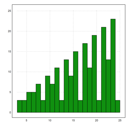
We compute a table of ranks.
>r=(3:24)'|0;
>for i=1 to rows(r); r[i,2]=rank(magic(r[i,1])); end;
>showlarge r
r =
     3      3
     4      3
     5      5
     6      5
     7      7
     8      3
     9      9
    10      7
    11     11
    12      3
    13     13
    14      9
    15     15
    16      3
    17     17
    18     11
    19     19
    20      3
    21     21
    22     13
    23     23
    24      3
>plot2d(r'[1],r'[2],>bar,>insimg);
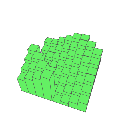
The following plot shows the structure of the 9x9 magic square.
>n=9; A=magic(n); plot3d(A/totalmax(A)*n/2,>bar,<frame, ...
   height=50°,angle=20°,>insimg);
Another example of Matlab used for integer computation. I think this is an abuse of the program. But I tried to do the example of Molder nevertheless.
The function char(x) works only for a single character. But chartostr(v) converts a vector of ASCII numbers.
>chartostr(48:57)
0123456789
>s=chartostr(32:96)
!"#$%&'()*+,-./0123456789:;<=>?@ABCDEFGHIJKLMNOPQRSTUVWXYZ[\]^_`
The built-in function strtochar() is the converse.
>strtochar(s)
[32, 33, 34, 35, 36, 37, 38, 39, 40, 41, 42, 43, 44, 45, 46, 47, 48,
49, 50, 51, 52, 53, 54, 55, 56, 57, 58, 59, 60, 61, 62, 63, 64, 65,
66, 67, 68, 69, 70, 71, 72, 73, 74, 75, 76, 77, 78, 79, 80, 81, 82,
83, 84, 85, 86, 87, 88, 89, 90, 91, 92, 93, 94, 95, 96]
Now the crypto algorithms maps pairs of letters to pairs.
![]()
>longformat; p=97
97
>x=[52;54]
                 52
                 54
>A=[71,2;2,26]
                 71                   2
                  2                  26
>y=mod(A.x,97)
                 17
                 53
>mod(A.y,97)
                 52
                 54
This function has its own inverse. The reason is the following.
>mod(A.A,97)
                  1                   0
                  0                   1
Here is a shorter version of the Matlab code.
>function crypto (s:string) ...
 global A,p;
 x=strtochar(s)-32;
 X=redim(x,2,(length(x)+1)/2);
 X=mod(A.X,p);
 x=redim(X,1,length(x))+32;
 return chartostr(x);
 endfunction
>s=crypto("Hello World")
H-?36 WZU{s
>crypto(s)
Hello World
>crypto(crypto("Hello World!"))
Hello World!
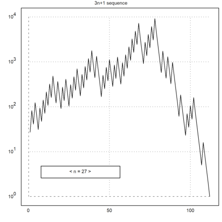
Another integer problem. It is not known, if the sequence
![]()
reaches 1 from all start values.
>function threenplus1 (n) ...
 N=n;
 repeat
   if mod(n,2)==0 then n=n/2; N=N|n;
   else n=3*n+1; N=N|n;
   endif
   until n==1;
 end;
 return N
 endfunction
>N=threenplus1(7)
[7,  22,  11,  34,  17,  52,  26,  13,  40,  20,  10,  5,  16,  8,  4,
2,  1]
>plot2d(N):
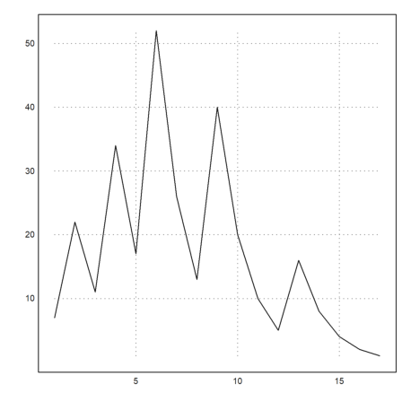
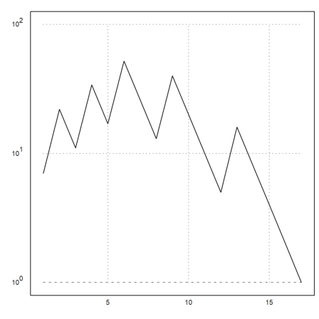
The values become large rather quickly. So it is best to use logarithmic plots.
>plot2d(N,>logplot):
Euler has an interfaces for interactions with the user.
>function test (n) ...
 N=threenplus1(n);
 plot2d(N,>logplot,title="3n+1 sequence");
 endfunction
>dragvalues("test","n",27,[7,107],100,0.5,0.8):
This is a section about floating point arithmetic. Here is the epsilon Euler uses for internal checks. It can be changed.
>longest epsilon
2.220446049250313e-012
It is 10000 times the smallest number such that 1+x is not x.
>printhex(epsilon)
2.7100000000000*16^-10
printhex() prints the hexadecimal representation of the IEEE number in Euler.
>printhex(2^-52)
1.0000000000000*16^-13
There is also a dual print.
>printdual(2^-52)
1.0000000000000000000000000000000000000000000000000000*2^-52
Note that 0.1 is not exactly representable.
>printhex(0.1)
1.999999999999A*16^-1
Thus adding 0.1 does not meet 1 exactly.
>x=0; loop 1 to 10; x=x+0.1; end; printdual(x)
1.1111111111111111111111111111111111111111111111111111*2^-1
However, the following works.
>0:0.1:1
[0, 0.1, 0.2, 0.3, 0.4, 0.5, 0.6, 0.7, 0.8, 0.9, 1]
As an example, the following expression does not evaluate to 0 exactly.
>longestformat; 1-(4/3-1)*3
2.220446049250313e-016
As a symbolic expression, it does.
>&1-(4/3-1)*3
0
In contrast to Matlab, Euler returns an error when solving the following linear system. The reason is the internal epsilon.
>[17,5;1.7,0.5]\[22;2.2]
Determinant zero!
Error in:
[17,5;1.7,0.5]\[22;2.2] ...
                       ^
The determinant is exactly 0. But we can find a best fit for solution.
>fit([17,5;1.7,0.5],[22;2.2])
      1.294117647058824
                      0
The following finds the fit among the fits that has minimal norm.
>svdsolve([17,5;1.7,0.5],[22;2.2])
      1.191082802547771
     0.3503184713375797
An interesting example is the evaluation of the following polynomial. First an exact plot.
>x = 0.988:.0001:1.012;
>plot2d(x,(x-1)^7,color=red,thickness=2):
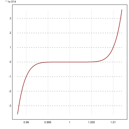
>p &= expand((x-1)^7)
          7      6       5       4       3       2
         x  - 7 x  + 21 x  - 35 x  + 35 x  - 21 x  + 7 x - 1
If we evaluated the expanded polynomial, we get lots of errors. Note that the y-scale is rather small.
>y = p(x);
>plot2d(x,y,color=blue,>add):
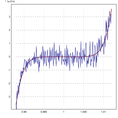
Euler has xpolyval(), which uses an exact residuum to iterate to the correct evaluation.
>longformat; p=polycons(ones(1,7))
[-1, 7, -21, 35, -35, 21, -7, 1]
>plot2d(x,xpolyval(p,x,eps=1e-16),color=red,thickness=2):

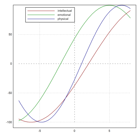
This is one of the exercises. Bio rhythm is of course nonsense. But it makes a great programming exercise.
>function bio (birth, now) ...
   t=linspace(now-8,now+8,200);
   plot2d(t-now,100*sin(2*pi/33*(t-birth)),color=red,);
   plot2d(t-now,100*sin(2*pi/28*(t-birth)),color=green,>add);
   plot2d(t-now,100*sin(2*pi/23*(t-birth)),color=blue,>add);
   labelbox(["intellectual","emotional","physical"],
     colors=[red,green,blue],x=0.5,w=0.4);
 endfunction
Today I am not at the height of my mental power. But emotionally, I am okay. So maybe this is the reason, why I tackle this irrational example.
>bio(day(1956,5,15),day(2012,14,7)):
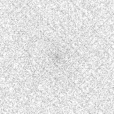
The Ulam spiral places the prime numbers in a spiral around the center of a rectangular grid. This is a demo from Molder's introduction.
We need to find the columns and rows of the n-th element in the spiral. That is essentially a programming exercise.
>function map col (n) ...
  if n==1 then return 0; endif;
  k=ceil(sqrt(n)); // on bounary of k*k square
  if mod(k,2)==0 then k=k+1; endif; // k must be odd
  d=n-(k-2)^2; // d-th element there
  u=(k^2-(k-2)^2)/4; // 4*u elements on this boundary
  k=(k-1)/2; // distance from center of the boundary
  if d<=u then return k;
  elseif d<=2*u then return k-(d-u);
  elseif d<=3*u then return -k;
  else return -k+(d-3*u)
  endif;
  endfunction
>function map row (n) ...
  if n==1 then return 0; endif;
  k=ceil(sqrt(n)); // on bounary of k*k square
  if mod(k,2)==0 then k=k+1; endif; // k must be odd
  d=n-(k-2)^2; // d-th element there
  u=(k^2-(k-2)^2)/4; // 4*u elements on this boundary
  k=(k-1)/2; // distance from center of the boundary
  if d<=u then return k-d;
  elseif d<=2*u then return -k;
  elseif d<=3*u then return -k+(d-2*u);
  else return k
  endif;
  endfunction
Once we have these functions, we need to test.
>function testspiral (n) ...
  k=2*n+1;
  A=zeros(k,k);
  c=col(1:k^2); r=row(1:k^2);
  for i=1 to k^2;
     A[r[i]+n+1,c[i]+n+1]=i;
  end;
  return A
  endfunction
>shortest testspiral(3)
    37     36     35     34     33     32     31
    38     17     16     15     14     13     30
    39     18      5      4      3     12     29
    40     19      6      1      2     11     28
    41     20      7      8      9     10     27
    42     21     22     23     24     25     26
    43     44     45     46     47     48     49
Seems to work.
>function makespiral (n) ...
  k=2*n+1;
  A=zeros(k,k);
  c=col(1:k^2); r=row(1:k^2);
  p=primes(k^2);
  for i=p;
     A[r[i]+n+1,c[i]+n+1]=1;
  end;
  return A
  endfunction
We test this. Note that we find the primes up to 251001 and generate a matrix of size 501x501. The matrix is then used like an image.
>A=makespiral(250);
>insrgb(rgb(!A,!A,!A));