by R. Grothmann
We investigate the stability of the BDF (backward differential formula) following the work of Gear e.a.
A BDF is a formula to solve differential equation. It uses multiple steps, and it is implicit. We assume the solution in the points x_0,...,x_n given as y_0,...,y_n and determine y_{n+1} implicitely such that
![]()
where p interpolations (x_i,y_i) for i=0,...n, and satisfies
![]()
First, let us determine the formula for p for the case n=1.
>function p(x) &= a+b*x+c*x^2;
It suffices to solve the special case
![]()
since we are only interested in equidistant discretization here.
>sol &= solve([p(-h)=y0,p(0)=y1,diffat(p(x),x=h)=yd2],[a,b,c])
                     h yd2 + 2 y1 - 2 y0      h yd2 - y1 + y0
       [[a = y1, b = -------------------, c = ---------------]]
                             3 h                      2
                                                   3 h
We define a function for the solution.
>function ps(x) &= p(x) with sol[1]
         2
        x  (h yd2 - y1 + y0)   x (- h yd2 - 2 y1 + 2 y0)
        -------------------- - ------------------------- + y1
                   2                      3 h
                3 h
The value of this function at h defines p(x_{n+1}) from the previous values and the derivative p'(x_{n+1}).
>function ystep(y0,y1,yd2,h) &= ps(h)|ratsimp
                         2 h yd2 + 4 y1 - y0
                         -------------------
                                  3
Here is an Euler function, which solves differential equations using this two step BDF. We use iteration for the solution of the non-linear equation
![]()
This is not optimal and must be replaced with faster solvers in real life.
>function bdf (f,a,b,n,y0) ...
   x=linspace(a,b,n);
   y=zeros(size(x));
   y[1:2]=runge(f,x[1:2],y0);
   h=(b-a)/n;
   for i=2 to n;
   y[i+1]=y[i]+f(x[i],y[i])*h;
   repeat
     yold=y[i+1];
     yd2=f(x[i+1],yold);
     y[i+1]=&:ystep(y[i-1],y[i],yd2,h);
     until yold~=y[i+1];
   end;
   end
   return y;
 endfunction
Let us show that the order of this procedure is 2.
>error1000=bdf("-2*x*y",0,1,1000,1)[-1]-1/E
4.9057824697e-007
>error2000=bdf("-2*x*y",0,1,2000,1)[-1]-1/E
1.22635597177e-007
>log(error1000/error2000)/log(2)
2.00010545601
Next, we solve the special equation
![]()
The non-linear problem for p can be solved explicitely for this equation. We get an explicit equation for y1 given y_0,y_1 to y_2.
>difgl &= solve(ystep(y0,y1,lambda*y2,h)=y2,y2)
                                y0 - 4 y1
                        [y2 = --------------]
                              2 h lambda - 3
Let us show for lambda=-5, that this recursion does indeed converge to the correct solution.
>lambda=-5; n=1000; h=1/n; ...
 sequence("(x[n-2]-4*x[n-1])/(2*h*lambda-3)",[1,exp(lambda/n)],n+1)[-1]
0.00673766561896
>exp(-5)
0.00673794699909
For stability, a formula must be able to solve this case, even if h*lambda is large. We want the iteration to converge to 0 for each lambda<0, or even better, for each complex lambda with re(lambda)<0. This is called A-stability.
The two step PDF is stable for this lambda and h, as we see with the following start values.
>sequence("(x[n-2]-4*x[n-1])/(2*h*lambda-3)",[1,0],n+1)[-1]
-0.00340277570995
>sequence("(x[n-2]-4*x[n-1])/(2*h*lambda-3)",[0,1],n+1)[-1]
0.0101912705026
We can study the problem exactly. The sequence of y_n is defined by a so-called difference formula. To solve such formulas, we can make the ansatz y_n=t^n. It follows easily, that solutions of this formula are determined by the zeros of
![]()
If t is a zero, t^n will satisfy the difference formula. We are interested to see |t|<1, if re(lambda*h)<0.
Replacing t=1/z, we seek the solutions of
![]()
We want to show that no |z| <= 1 with re(p(z))<0 exists.
>function q(z) &= 3-4*z+z^2
                              2
                             z  - 4 z + 3
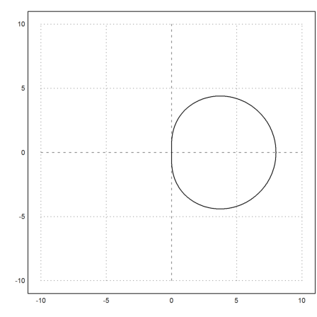
Let us plot the image of |z|=1. We see that indeed, the method is A-stable, since the interior of the image is in the right half plane.
>z=exp(I*linspace(0,2pi,1000)); plot2d(q(z),r=10):
Discussing that involves a discussion of the function
>&realpart(q(cos(x)+I*sin(x)))|trigsimp
                       2         2
                  - sin (x) + cos (x) - 4 cos(x) + 3
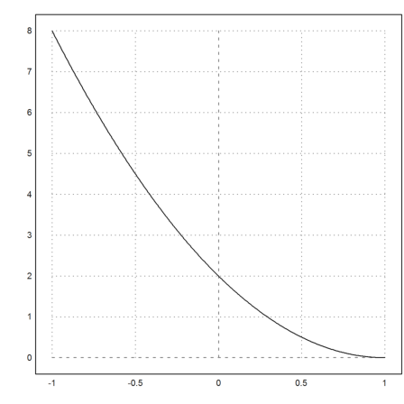
We can do that analytically, but here is a simple plot.
>plot2d("2*x^2-4*x+2",-1,1):
Next we do the same for the three term BDF.
>function p(x) &= a+b*x+c*x^2+d*x^3;
>sol &= solve([p(-2*h)=y0,p(-h)=y1,p(0)=y2,diffat(p(x),x=h)=yd3],[a,b,c,d]);
>function ps(x) &= p(x) with sol[1];
>function ystep(y0,y1,y2,yd3,h) &= ps(h)|ratsimp
                    6 h yd3 + 18 y2 - 9 y1 + 2 y0
                    -----------------------------
                                 11
>sol &= solve(ystep(y0,y1,y2,lambda*y3,h)=y3,y3)
                           - 18 y2 + 9 y1 - 2 y0
                     [y3 = ---------------------]
                              6 h lambda - 11
The formula for
![]()
has three terms now. We follow the same ideas as above.
>function q(z) &= 11+(num(rhs(sol[1])) with [y0=z^3,y1=z^2,y2=z])
                           3      2
                      - 2 z  + 9 z  - 18 z + 11
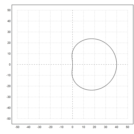
This polynomial now stretches into the left half plane. This makes the method unstable for h*lambda=i.
>plot2d(q(z),r=50):
We derive an instable and unusable formula. The idea is to interpolate
![]()
![]()
using Hermite interpolation, then to set
![]()
>function p(x) &= a+b*x+c*x^2+d*x^3
                           3      2
                        d x  + c x  + b x + a
>sol &= solve( ...
   [p(-h)=y0,diffat(p(x),x=-h)=yd0,p(0)=y1,diffat(p(x),x=0)=yd1],[a,b,c,d])
                               h (2 yd1 + yd0) - 3 y1 + 3 y0
        [[a = y1, b = yd1, c = -----------------------------,
                                             2
                                            h
                                         h (yd1 + yd0) - 2 y1 + 2 y0
                                     d = ---------------------------]]
                                                      3
                                                     h
We can easily derive a formula for the next y-value.
>function ystep(y0,yd0,y1,yd1,h) &= p(h) with sol[1]
h (2 yd1 + yd0) + h (yd1 + yd0) + h yd1 - 4 y1 + 5 y0
To investigate the stability, we use y'=lambda*y as above.
>y2 &= ystep(y0,lambda*y0,y1,lambda*y1,h)
        h (2 y1 lambda + y0 lambda) + h (y1 lambda + y0 lambda)
                                           + h y1 lambda - 4 y1 + 5 y0
Set h*lambda=c.
>y2c &= ratsimp(y2 with lambda=c/h)
(4 c - 4) y1 + (2 c + 5) y0
This difference recursion should be stable for re(c)<0. So let us investigate this.
>&c with solve(y2n-y2c,c), function h(t) &= % with [y2n=t^2,y1=t,y0=1]
                          y2n + 4 y1 - 5 y0
                          -----------------
                             4 y1 + 2 y0


                              2
                             t  + 4 t - 5
                             ------------
                               4 t + 2
We now do not want to have values |x| > 1, which touch the negative axis.
>z=exp(I*linspace(0,2pi,1000)); ...
 plot2d(h(z),r=6):
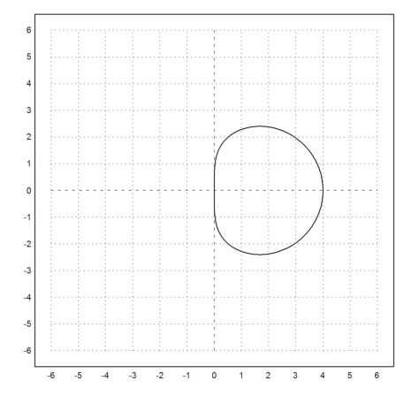
But we see that such x exist for all c with re(c)<0. Indeed, the algorithm fails completely, even for moderate c.
>lambda=-1; n=100; h=1/n; c=lambda*h
-0.01
>y=sequence("(2c+5)*x[n-1]+(4c-4)*x[n-2]",[1,exp(-lambda*h)],n+1)[-1]
-2.03142847388e+057